Applied Linear Models

STAT3530 Fall 2026

Does insulation reduce energy use?

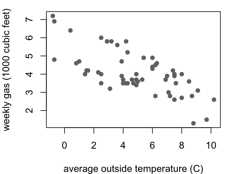
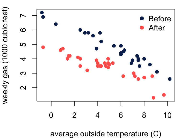
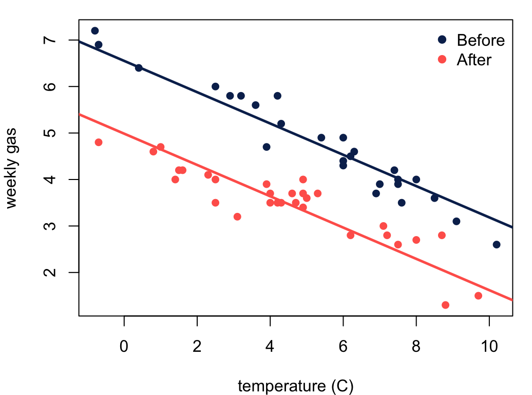
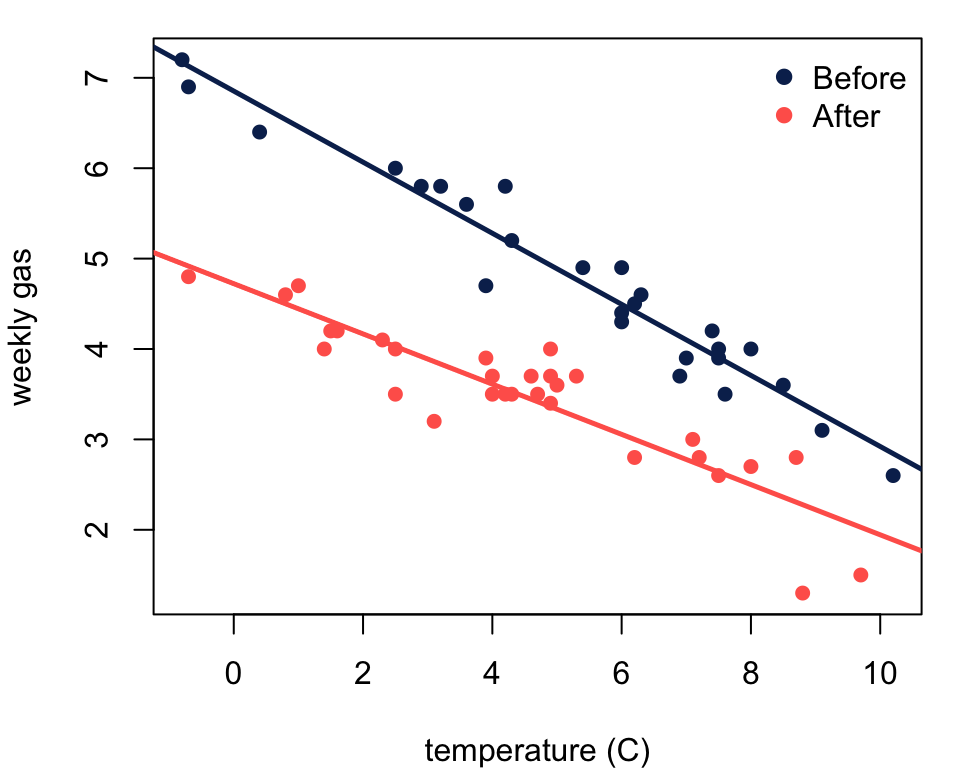
Weekly gas use and average outside temperature over 56 weeks.

Between heating seasons, the home underwent cavity-wall insulation.

Looks like there’s an effect. How do we quantify it?

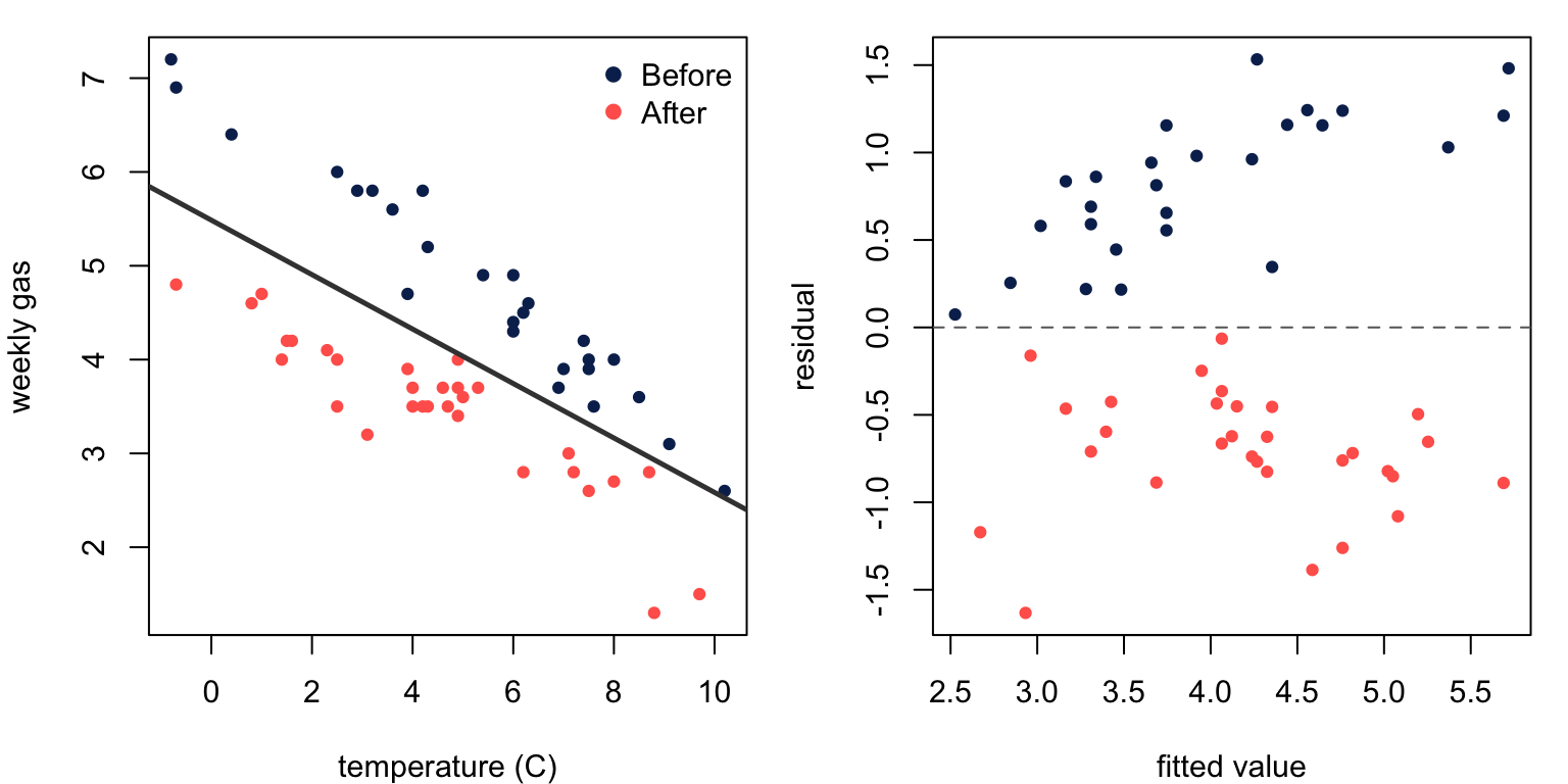
A model without insulation

A simple linear regression misses obvious structure.

Idea: add insulation as a predictor. \[ \text{gas}_i = \beta_0 + \beta_1\,\text{temp}_i + \beta_2\,\text{insulation}_i + \epsilon_i \]

Issue: \(\beta_2 \times \text{Before} =\; ?\)

You have seen this before

Midterm: \(Y = X\beta + \epsilon\) where \[X = \left[\begin{array}{cc} 1 &0 \\ \vdots &\vdots \\ 1 &0 \\ 1 &1 \\ \vdots &\vdots \\ 1 &1\end{array}\right] \begin{matrix} \left.\vphantom{\begin{matrix}1\\ \vdots\\ 1\end{matrix}}\right\} \; n_0 = 47 \,\text{females}\\[0.6em] \left.\vphantom{\begin{matrix}1\\ \vdots\\ 1\end{matrix}}\right\} \; n_1 = 97 \,\text{males} \end{matrix}\]

Here the explanatory variable encodes the categorical variable sex:

• \(x_i = 1\) for male cats
• \(x_i = 0\) for female cats

SLR with one categorical predictor

\[ \text{bwt}_i = \beta_0 + \beta_1\,\text{sex}_i + \epsilon_i \]

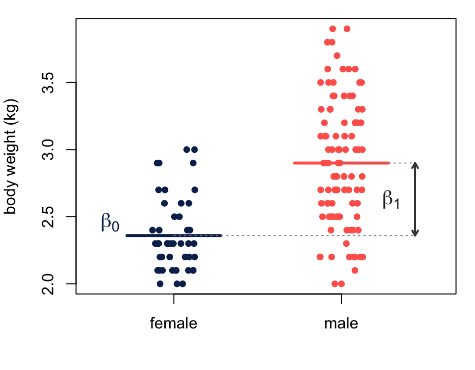
For female cats, \(\text{sex} = 0\) and \[\mathbb{E}[\text{bwt}] = \beta_0\]

For male cats, \(\text{sex} = 1\) and \[\mathbb{E}[\text{bwt}] = \beta_0 + \beta_1\]

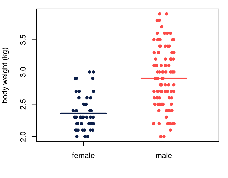
So the coefficient \(\beta_1\) is the difference in group means.

Factors in R

Categorical variables appear either as factors or character strings. Compare:

# string
str(cats$sex.chr)

 chr [1:144] "F" "F" "F" "F" "F" "F" "F" "F" "F" "F" "F" "F" "F" "F" "F" ...

# factor
str(cats$sex.fct)

 Factor w/ 2 levels "F","M": 1 1 1 1 1 1 1 1 1 1 ...

lm() handles both naturally

# string
lm(bwt ~ sex.chr, data = cats) |> coef()

(Intercept)    sex.chrM 
  2.3595745   0.5404255 

# factor
lm(bwt ~ sex.fct, data = cats) |> coef()

(Intercept)    sex.fctM 
  2.3595745   0.5404255 

In this case, F is the reference level, meaning that \(x_i = 0\) encodes F.

• mean body weight for female cats is \(2.36\) kg
• mean body weight for male cats is \(2.36 + 0.54 = 2.90\) kg

Factor encodings

We can check how R interprets the categorical variable.

# check factor encoding
contrasts(cats$sex.fct)

  M
F 0
M 1

This shows one variable, called M, that encodes F = 0 and M = 1.

But only works for factors.

# won't work with strings
contrasts(cats$sex.chr)

Error in `contrasts()`:
! contrasts apply only to factors

So what R does under the hood if you supply lm() with a string is convert to a factor with the alphabetically first level as the reference.

# convert to factor
as.factor(cats$sex.chr) |> contrasts()

  M
F 0
M 1

# note 'a' becomes reference
as.factor(c('b', 'a')) |> contrasts()

  b
a 0
b 1

Spot the issue

Why not specify a model that encodes the factor with two indicators?

\[ \text{bwt}_i = \beta_0 + \beta_1\,\text{F}_i + \beta_2\,\text{M}_i + \epsilon_i \quad\text{so that}\quad X = \left[\begin{array}{ccc} 1 &1 &0 \\ \vdots &\vdots &\vdots \\ 1 &1 &0 \\ 1 &0 &1 \\ \vdots &\vdots &\vdots \\ 1 &0 &1\end{array}\right] \]

The indicators sum to the intercept column, so \(X\) is not full rank.

Aside. But you could drop the intercept and specify the model: \[ \text{bwt}_i = \beta_1\,\text{F}_i + \beta_2\,\text{M}_i + \epsilon_i \] So there are other possible encodings. We will see more in ANOVA.

An energy use model

Encode the insul variable: reference level is Before.

# factor encoding for insulation
contrasts(whiteside$insul)

       After
Before     0
After      1

Now add it to the model:

\[ \text{gas}_i = \beta_0 + \beta_1 \text{temp}_i + \beta_2 \text{insul}_i + \epsilon_i \]

# fit with categorical predictor
fit <- lm(gas ~ temp + insul, data = whiteside)
coef(fit)

(Intercept)        temp  insulAfter 
   6.551329   -0.336697   -1.565205 

Note that this is a single model that describes two parallel lines.

Coefficient interpretation

\[ \text{gas}_i = \beta_0 + \beta_1 \text{temp}_i + \beta_2 \text{insul}_i + \epsilon_i \] Consider what happens to the model equation for each group:

• \(\text{insul} = 0 \quad\Rightarrow\quad \mathbb{E}[\text{gas}] = \beta_0 + \beta_1 \text{temp}\)
• \(\text{insul} = 1 \quad\Rightarrow\quad \mathbb{E}[\text{gas}] = (\beta_0 + \beta_2) + \beta_1 \text{temp}\)

So:

• \(\beta_1\) describes the association with \(\text{temp}\) across both groups
• \(\beta_0\) is the intercept for the reference group (before insulation)
• \(\beta_0 + \beta_2\) is the intercept for the other group (after insulation)

And thus \(\beta_2\) is the difference in means, i.e., the effect of insulation.

Inference

What is the effect of insulation on mean gas consumption for this house?

Easy to answer with a confidence interval.

# confidence interval
confint(fit)['insulAfter', ]

    2.5 %    97.5 % 
-1.759869 -1.370540 

With 95% confidence, insulation is estimated to lower mean gas consumption by between 1,371 and 1,760 cubic feet per week at any given time in the season.

Remark. The causal interpretation only works if we assume no interannual effects and no unmeasured confounding.

Different slopes

Two (equivalent) reasons to consider different slopes here:

1. the effect of insulation could depend on external temperature
2. the association between temperature and gas use might change with insulation

To allow this, we add an interaction, or product term, between temperature and insulation:

\[\text{gas}_i = \beta_0 + \beta_1 \text{temp}_i + \beta_2 \text{insul}_i + \beta_3 (\text{temp}_i \times \text{insul}_i) + \epsilon_i\]

Now rewriting the model equation by group gives

• \(\text{insul} = 0 \quad\Rightarrow\quad \mathbb{E}[\text{gas}] = \beta_0 + \beta_1 \text{temp}\)
• \(\text{insul} = 1 \quad\Rightarrow\quad \mathbb{E}[\text{gas}] = (\beta_0 + \beta_2) + (\beta_1 + \beta_3) \text{temp}\)

So \(\beta_2\) is the difference in intercepts, and \(\beta_3\) is the difference in slopes.

Fitting with interactions

Two ways, syntactically, via lm():

lm(gas ~ temp * insul, data = whiteside)
lm(gas ~ temp + insul + temp:insul, data = whiteside)

Algebraically, the model matrix here is: \[X = \left[\begin{array}{cccc} 1 &x_1 &0 &0 \\ \vdots &\vdots &\vdots &\vdots \\ 1 &x_{26} &0 &0 \\ 1 &x_{27} &1 &x_{27} \\ \vdots &\vdots &\vdots &\vdots \\ 1 &x_{56} &1 &x_{56} \end{array}\right]\]

Check some example rows:

   (Intercept) temp insulAfter temp:insulAfter
1            1 -0.8          0             0.0
2            1 -0.7          0             0.0
27           1 -0.7          1            -0.7
28           1  0.8          1             0.8

Do the slopes differ?

Check the partial test on \(\beta_3\):

fit.int <- lm(gas ~ temp * insul, data = whiteside)
summary(fit.int)$coefficients

                  Estimate Std. Error    t value     Pr(>|t|)
(Intercept)      6.8538277 0.13596397  50.409146 7.997414e-46
temp            -0.3932388 0.02248703 -17.487358 1.976009e-23
insulAfter      -2.1299780 0.18009172 -11.827185 2.315921e-16
temp:insulAfter  0.1153039 0.03211212   3.590665 7.306852e-04

Interpretation 1: group difference depends on continuous predictor

The data provide evidence that the effect of insulation depends on temperature.

Interpretation 2: association depends on group

The data provide evidence that the association between gas consumption and temperature depends on insulation.

Both are correct, but I favor the first in this case.

Inference, revisited

So now what is the effect of insulation?

The difference in means now depends on temperature \(t\): \[ \underbrace{(\beta_0 + \beta_2) + (\beta_1 + \beta_3)\;t}_{\mathbb{E}[\text{gas}] \text{ when } \text{insul} = 1} - \underbrace{\beta_0 + \beta_1\;t}_{\text{when } \text{insul} = 0} = \beta_2 + \beta_3\; t \]

For fixed \(t\), this is a contrast: \[ c^T\beta \quad\text{where}\quad c^T = \left[\begin{array}{cccc} 0 &0 &1 &t\end{array}\right] \]

Recentering at \(t\) makes \(\beta_2\) the desired contrast:

at <- function(t) {
  fit <- lm(gas ~ I(temp - t) * insul, data = whiteside)
  confint(fit)['insulAfter', ]
}

tvals <- c(0, 2.5, 5, 7.5, 10)
round(cbind(t = tvals, t(sapply(tvals, at))), 3)

        t  2.5 % 97.5 %
[1,]  0.0 -2.491 -1.769
[2,]  2.5 -2.076 -1.608
[3,]  5.0 -1.730 -1.377
[4,]  7.5 -1.508 -1.022
[5,] 10.0 -1.350 -0.604

So the estimated effect is larger at lower temperature.

Many levels

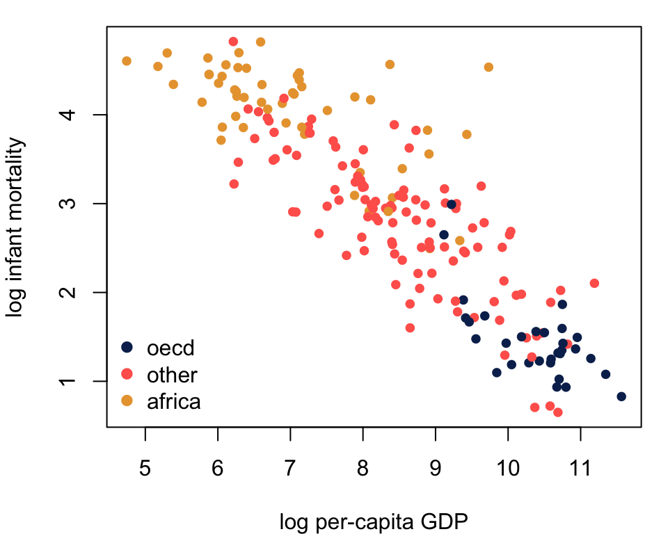
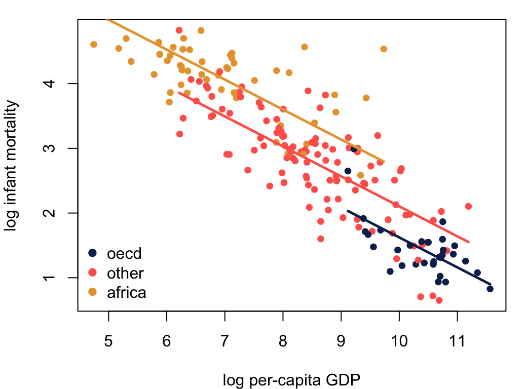
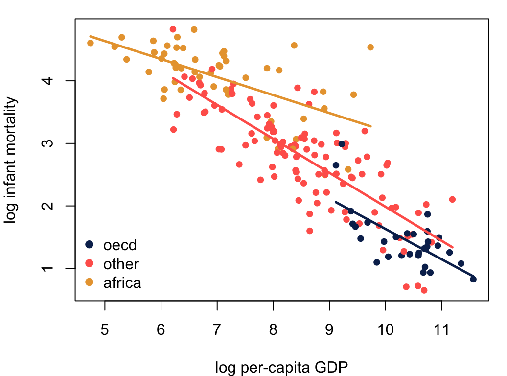
Infant mortality and per-capita GDP for 193 countries:

• 31 OECD countries
• 52 African countries
• 110 other countries

Does infant mortality differ by region after accounting for national income?

Two indicators for three levels

Now oecd is the reference level, and one indicator encodes each of the other levels:

contrasts(un$group)

       other africa
oecd       0      0
other      1      0
africa     0      1

The model without interactions (i.e., parallel lines) is:

\[\log(\text{mort}_i) = \beta_0 + \beta_1 \log(\text{gdp}_i) + \beta_2\,\text{other}_i + \beta_3\, \text{africa}_i + \epsilon_i\]

Interpretation are relative to the reference level:

• \(\beta_2\) is the difference in means between other and oecd countries
• \(\beta_3\) is the difference in means between africa and oecd countries

The parallel lines model

lm(lmort ~ lgdp + group, data = un) |>
  coef()

(Intercept)        lgdp  groupother groupafrica 
  6.2550828  -0.4631826   0.4801703   1.0491120 

Estimates suggest higher mortality in African and non-OECD countries.

• other: \(e^{0.48} = 1.6\)-fold increase
• africa: \(e^{1.05} = 2.9\)-fold increase

This particular comparison may be a little unreliable since GDP ranges also differ.

Inference with multiple levels

Here, partial \(t\) tests on indicators test pairwise comparisons with the reference level.

fit <- lm(lmort ~ lgdp + group, data = un) 
summary(fit)$coef

              Estimate Std. Error    t value     Pr(>|t|)
(Intercept)  6.2550828 0.32500043  19.246383 2.068539e-46
lgdp        -0.4631826 0.03030728 -15.282882 7.389495e-35
groupother   0.4801703 0.11003259   4.363891 2.099843e-05
groupafrica  1.0491120 0.14677408   7.147801 1.867312e-11

Each group differs significantly from oecd.

But testing whether the categorical variable is a significant predictor requires an \(F\) test

lm(lmort ~ lgdp, data = un) |>
  anova(fit)

Analysis of Variance Table

Model 1: lmort ~ lgdp
Model 2: lmort ~ lgdp + group
  Res.Df    RSS Df Sum of Sq      F    Pr(>F)    
1    191 53.272                                  
2    189 41.239  2    12.032 27.572 3.113e-11 ***
---
Signif. codes:  0 '***' 0.001 '**' 0.01 '*' 0.05 '.' 0.1 ' ' 1

The data provide evidence that median infant mortality differs by country group after adjusting for national income.

Including interactions

Same as before, but with (a lot) more terms:

\[ \text{lmort}_i = \beta_0 + \beta_1\,\text{lgdp}_i + \beta_2\,\text{oth}_i + \beta_3 \,\text{afr}_i + \beta_4 (\text{lgdp}_i \times \text{oth}_i) + \beta_5 (\text{lgdp}_i \times \text{afr}_i) + \epsilon_i \]

The model equation, by group:

group	intercept	slope
oecd	\(\beta_0\)	\(\beta_1\)
other	\(\beta_0 + \beta_2\)	\(\beta_1 + \beta_4\)
africa	\(\beta_0 + \beta_3\)	\(\beta_1 + \beta_5\)

fit.int <- lm(lmort ~ lgdp * group, data = un)

Testing interactions

Now the interaction involves multiple terms, and slopes differ if either \(\beta_4 \neq 0\) or \(\beta_5 \neq 0\).

So we conduct an \(F\) test of the hypothesis \[ H_0: \beta_4 = \beta_5 = 0 \]

anova(fit, fit.int)

Analysis of Variance Table

Model 1: lmort ~ lgdp + group
Model 2: lmort ~ lgdp * group
  Res.Df    RSS Df Sum of Sq      F    Pr(>F)    
1    189 41.239                                  
2    187 38.042  2    3.1972 7.8579 0.0005287 ***
---
Signif. codes:  0 '***' 0.001 '**' 0.01 '*' 0.05 '.' 0.1 ' ' 1

The slopes differ.

Changing the reference

The partial tests reflect that neither group differs from the reference.

round(summary(u2)$coefficients, 4)

                 Estimate Std. Error t value Pr(>|t|)
(Intercept)        6.4764     1.3384  4.8390   0.0000
lgdp              -0.4845     0.1290 -3.7576   0.0002
groupother         0.9429     1.3746  0.6859   0.4936
groupafrica       -0.4005     1.3908 -0.2879   0.7737
lgdp:groupother   -0.0589     0.1340 -0.4392   0.6610
lgdp:groupafrica   0.1966     0.1395  1.4091   0.1605

So the \(F\) test must be picking up the difference between other and africa.

Change the reference and the partial tests capture the difference.

un2 <- transform(un, group = relevel(group, ref = 'africa'))
fit <- lm(lmort ~ lgdp * group, data = un2)
round(summary(fit)$coef, 4)

                Estimate Std. Error t value Pr(>|t|)
(Intercept)       6.0759     0.3784 16.0573   0.0000
lgdp             -0.2880     0.0532 -5.4094   0.0000
groupoecd         0.4005     1.3908  0.2879   0.7737
groupother        1.3433     0.4913  2.7342   0.0069
lgdp:groupoecd   -0.1966     0.1395 -1.4091   0.1605
lgdp:groupother  -0.2554     0.0645 -3.9607   0.0001