The corresponding population hypothesis is the model constraint
\[
H_0: \theta(\beta) = 2
\qquad\Longleftrightarrow\qquad
\{\beta: |\beta_2| \geq |\beta_k| \text{ for each } k > 0\}
\]
But this defines a (nonconvex) cone, not a subspace, so you can’t do F tests.
Inference by model-based simulation
Simulation based inference builds a sampling distribution empirically via computation.
The basic idea:
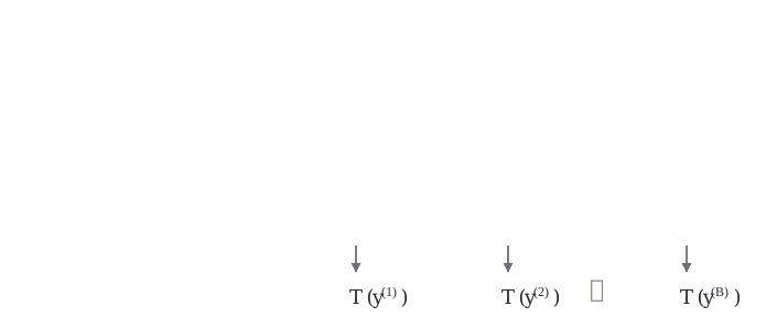
simulate many datasets under a fitted model
compute a test statistic for each simulated dataset
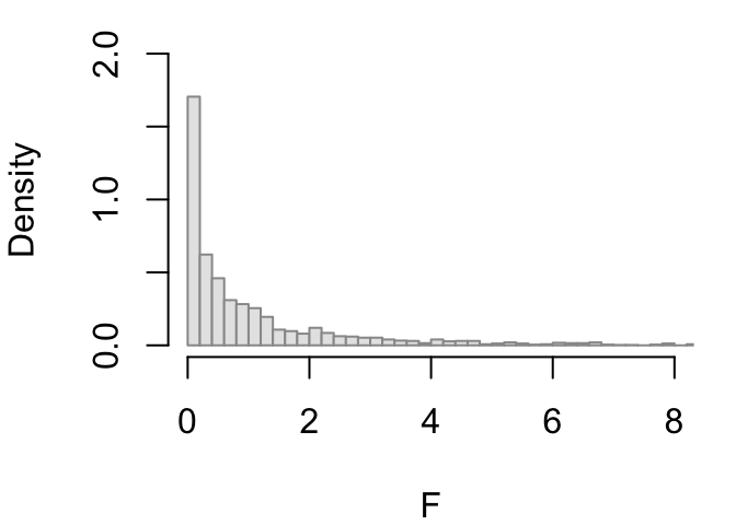
construct a frequency distribution
This is flexible and largely theory free, but it can be tricky to figure out how to simulate from an appropriate model.
Randomization in regression
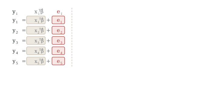
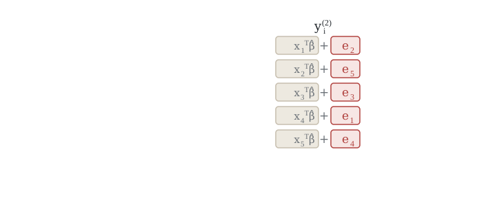
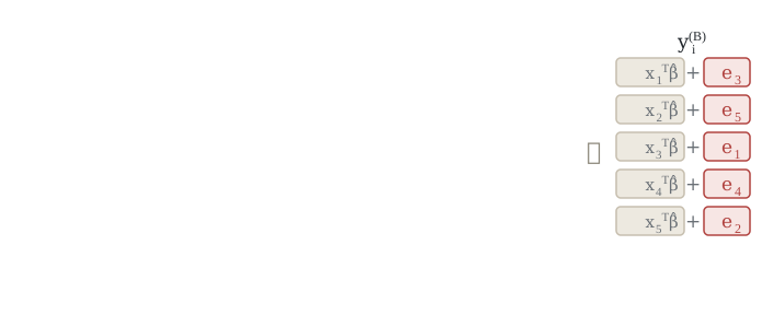
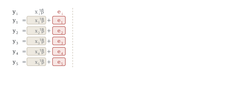
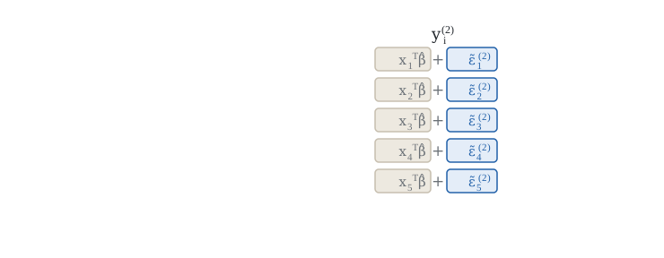
One approach: fit a model (possibly under \(H_0\)), shuffle residuals to simulate new data.
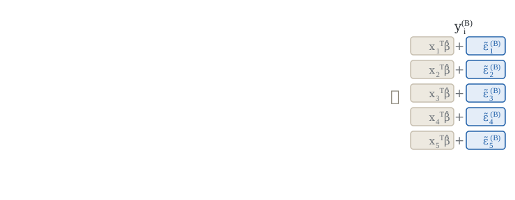
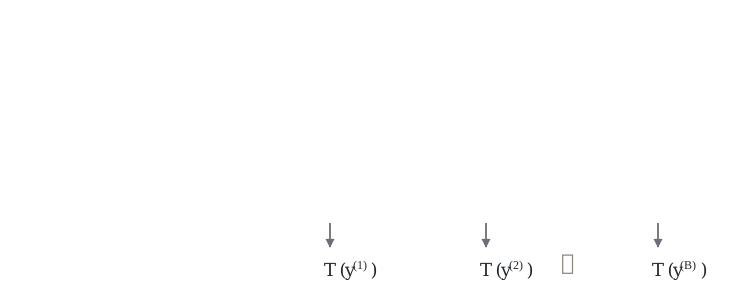
Do this many (say \(B = 1000\)) times, then build a sampling distribution for any \(T(Y)\).
F test by randomization
Recall the contrast \(H_0: \beta_2 = \beta_3\) in the cheddar model. Here’s a randomization test:
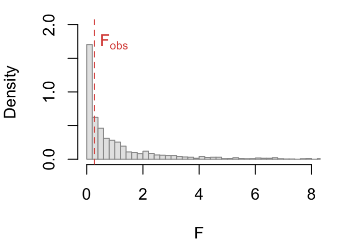
# constrained fit and the observed F statisticfit.c <-lm(taste ~ Acetic +I(H2S + Lactic), data = cs)F.obs <-anova(fit.c, fit.s)$F[2]# recompute the F stat from new datasim.F <-function(y) { m0 <-lm(y ~ Acetic +I(H2S + Lactic), data = cs) m1 <-lm(y ~ Acetic + H2S + Lactic, data = cs)anova(m0, m1)$F[2]}# shuffle residuals 2000 timesset.seed(1)F.null <-replicate(2000, { yb <-fitted(fit.c) +sample(resid(fit.c))sim.F(yb)})
# randomization p valuemean(F.null >= F.obs)
[1] 0.6065
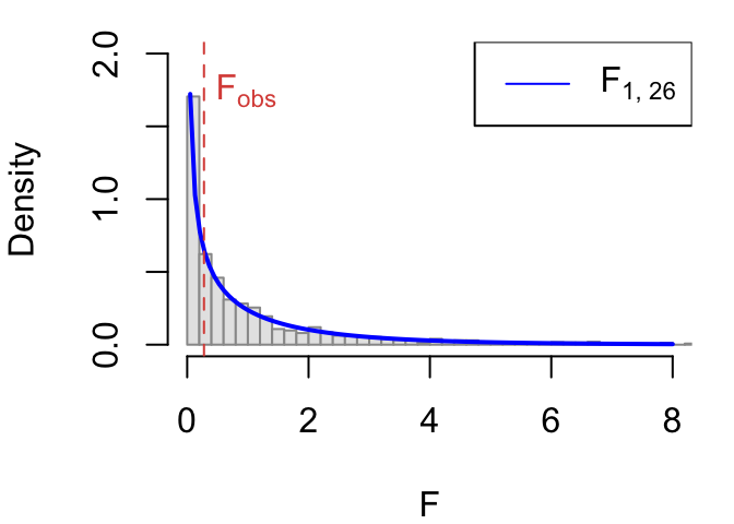
# compare with the parametric testanova(fit.c, fit.s)$Pr[2]
[1] 0.6031142
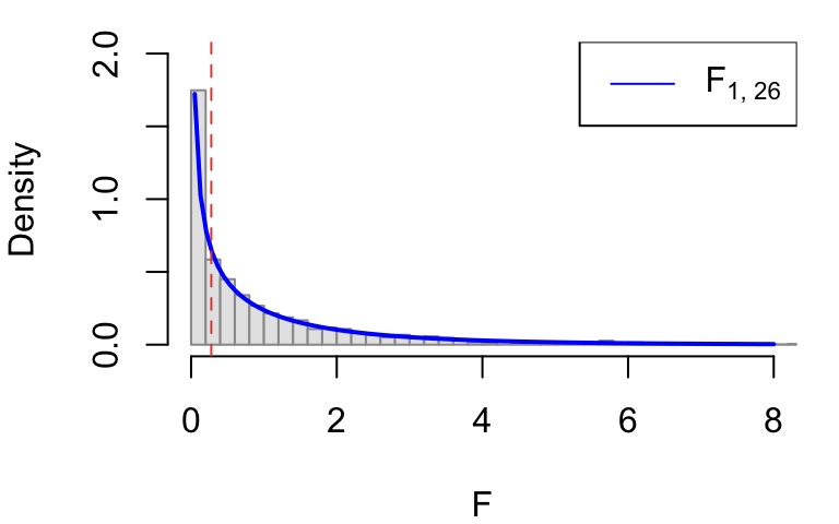
Here we’re just approximating the F distribution, so the tests are almost identical.
Parametric bootstrap
Another approach: draw new residuals from the fitted error model \(\tilde\epsilon_i \stackrel{iid}{\sim} N(0, \hat\sigma^2)\).
As before, set \(B\) large and build a sampling distribution for \(T(Y)\).
This is called a “parametric” bootstrap because we are drawing from an error model.
Bootstrap F test
Testing the same contrast in the cheddar model:
# draw new residuals 2000 timesset.seed(1)F.boot <-replicate(2000, { yb <-fitted(fit.c) +rnorm(30, 0, sigma(fit.c))sim.F(yb)})# bootstrap p valuemean(F.boot >= F.obs)
[1] 0.607
We are again just approximating the theoretical sampling distribution.
However the bootstrap distribution is a bit closer to theory since it assumes normality.
Nonstandard inference
Where model-based simulation really shines is for unusual estimands.
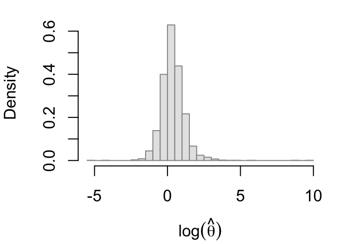
Let’s estimate how often the data ranks H2S as most important to taste: \[
P\left(\theta(\hat{\beta}) = 2\right)
\qquad\text{where}\qquad
\theta(\beta) = \text{argmax}_{j>0}\; |\beta_j|
\]
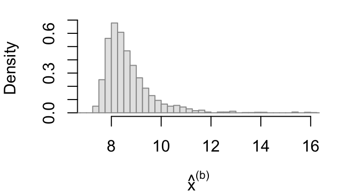
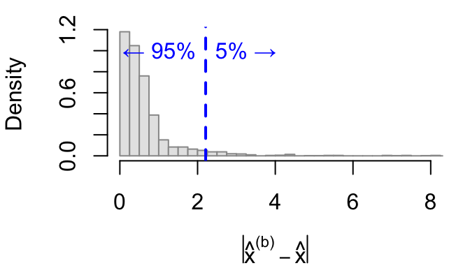
With 95% confidence, the level of state spending required (in 1994-1995) to achieve a mean SAT total of 975 is estimated to be between $7571 and $11,308.
Note that the interval is not symmetric about the point estimate:
# point estimatex.star(sat.fit, y0 =975, tk =30)
(Intercept)
   8.434961
Methods of interval construction
The symmetry of the usual parametric confidence intervals comes from the normal sampling distribution.
In principle, one could substitute a bootstrap standard error:
But note it forces the lower bound outside the observed range.
A nonlinear relationship
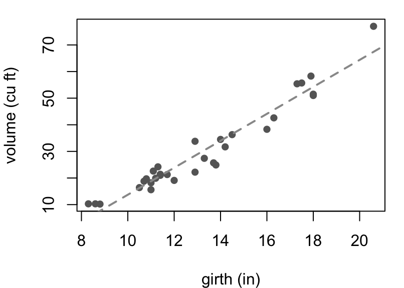
Recall the tree girth data.
# fit a simple linear modelm0 <-lm(Volume ~ Girth, data = trees)
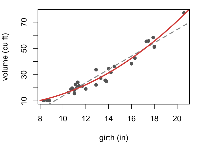
Girth is a circumference. By geometry: \[\text{volume} \propto \text{girth}^2\]
So simply add a quadratic term and fit \[
\text{volume}_i = \beta_0 + \beta_1\, \underbrace{\text{girth}_i}_{f_1(x_i)} + \beta_2\,\underbrace{\text{girth}_i^2}_{f_2(x_i)} + \epsilon_i
\]
# fit a polynomial modelm1 <-lm(Volume ~ Girth +I(Girth^2), data = trees)
And we can test for a quadratic relationship.
# test for quadratic relationshipanova(m0, m1)$`Pr(>F)`[2]
[1] 0.000152389
Polynomial models
More broadly, we can fit a \(k^\text{th}\) order polynomial via \[
Y_i = \beta_0 + \beta_1\,x_i + \beta_2\,x_i^2 + \cdots + \beta_k\,x_i^k + \epsilon_i
\]
For example, we could try a cubic model for the girth data.
# cubic modelm2 <-lm(Volume ~poly(Girth, degree =3), data = trees)# test comparing cubic and quadratic modelsanova(m1, m2)
Analysis of Variance Table

Model 1: Volume ~ Girth + I(Girth^2)
Model 2: Volume ~ poly(Girth, degree = 3)
  Res.Df    RSS Df Sum of Sq      F Pr(>F)
1     28 311.38
2     27 302.18  1    9.2022 0.8222 0.3726
No evidence of a cubic relationship.
Aside: poly() in R
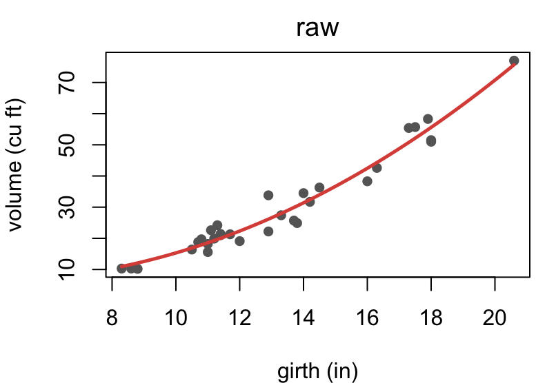
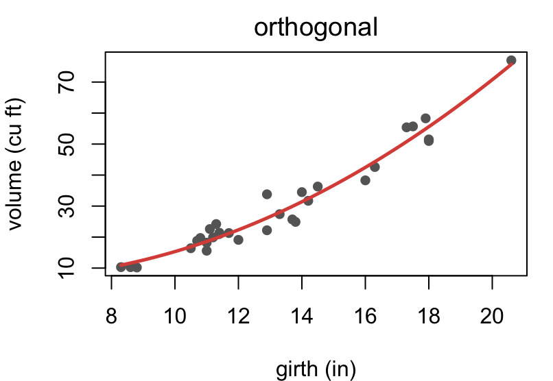
The poly() function generates polynomials.
head(trees$Girth, 3)
[1] 8.3 8.6 8.8
# "raw" quadratic termspoly(trees$Girth, degree =2, raw = T) |>head(3)
Gram Schmidt orthogonalization gives \(X \to XT\) where \(T\) is an invertible upper-triangular matrix, so \(\text{col}(XT) = \text{col}(X)\) and the least squares projections are identical.
In other words, different coordinates, same column space.
Ozone in LA
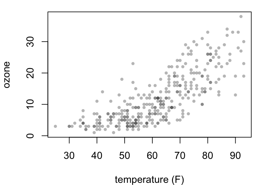
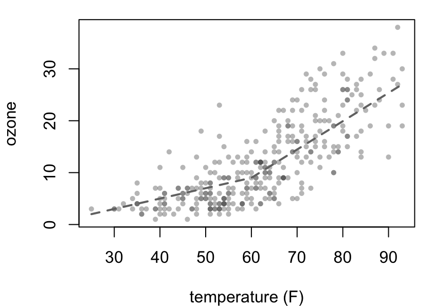
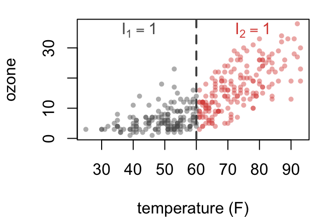
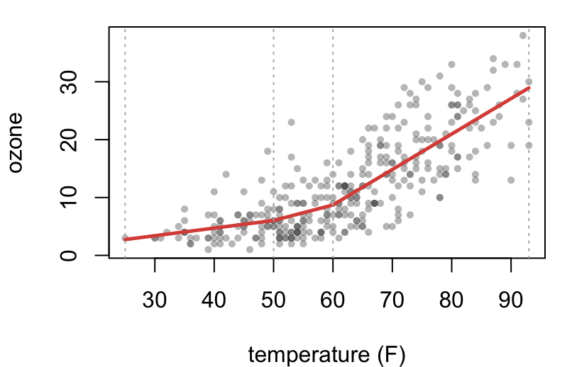
Ozone concentration against temperature, 330 days in the Los Angeles basin.
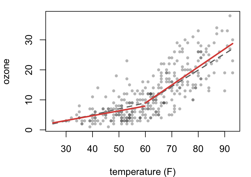
The data seem to show a change point around 60\(^\circ\)F.
Could fit two modelsBut better if continuous
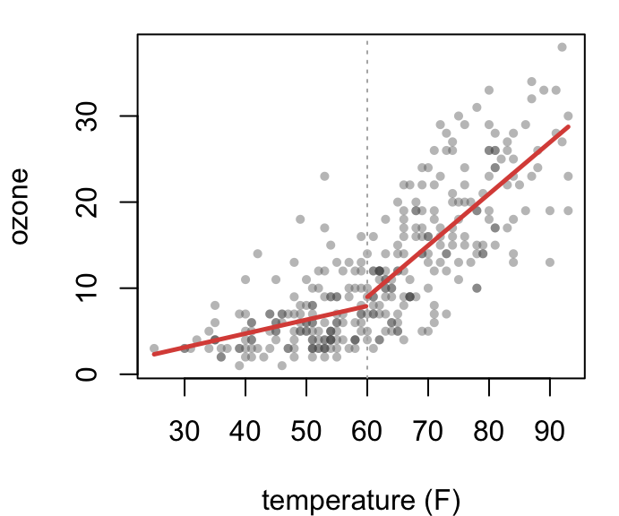
A piecewise linear model \[
Y_i =
\begin{cases}
\beta_0 + \beta_1 x_i + \epsilon_i &\text{if } x_i \leq t \\
\alpha_0 + \alpha_1 x_i + \epsilon_i &\text{if } x_i > t
\end{cases}
\] with the usual assumptions on \(\epsilon_i\).
Knots
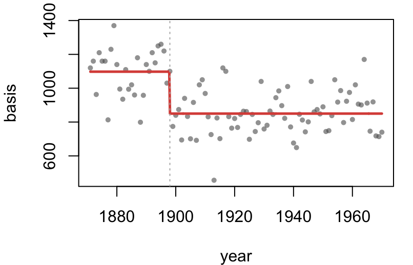
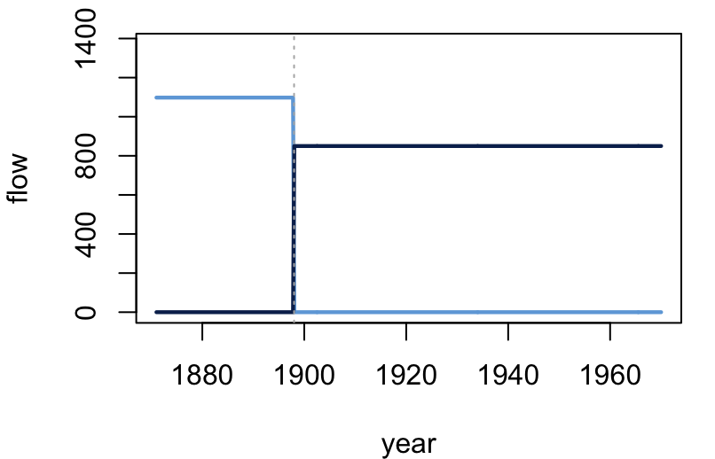
Cut the range at a knot\(t\) via indicator functions:
\[\begin{align*}
I_1(x) &= \begin{cases} 1, &x \leq t \\ 0, &x > t \end{cases}
\qquad
I_2(x) = \begin{cases} 1, &x > t \\ 0, &x \leq t \end{cases}
\end{align*}\]
So the estimates are \[
\hat\beta_0 = -1.69
\qquad
\hat\beta_1 = 0.16
\qquad
\hat\alpha_0 = -27.00
\qquad
\hat\alpha_1 = 0.60
\]
Making ends meet
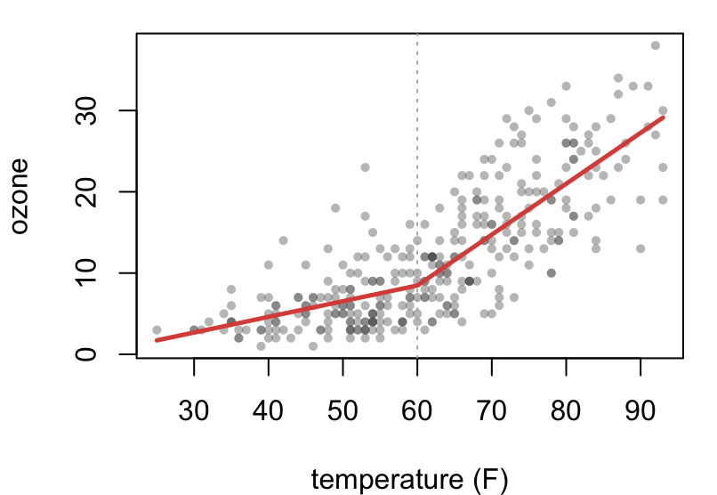
Let’s add a constraint that the mean has to be continuous in \(x\)
\[
\underbrace{\beta_0 + \beta_1 t}_{\text{left piece at } t}
\;=\;
\underbrace{\alpha_0 + \alpha_1 t}_{\text{right piece at } t}
\quad\Longleftrightarrow\quad
\beta_0 + \beta_1 t - \alpha_0 - \alpha_1 t = 0
\]
This is a contrast! \[
c^T\left[\begin{array}{c} \beta \\ \alpha \end{array}\right] = 0
\quad\text{where}\quad
c^T = [\,1\;\;t\;\;-1\;\;-t\,]
\]
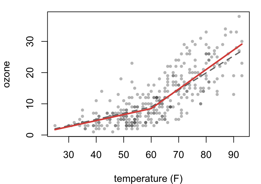
We can reparametrize under the contrast to obtain the “broken stick” model \[
Y_i = \gamma_0 + \gamma_1\,x_i + \gamma_2\, (x_i - t)_+ + \epsilon_i
\quad\text{where}\quad
(x_i - t)_+ = \max(x_i - t, 0)
\]
A bit of algebra and you can show \[
\gamma_0 = \beta_0
\quad
\gamma_1 = \beta_1
\quad
\underbrace{\gamma_2 = \alpha_1 - \beta_1}_\text{change in slope at knot}
\]
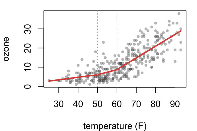
Each \((x - t_k)_+\) is flat to the left of its knot, so only changes the slope past \(t_k\).
For example, a broken stick model with \(K = 2\) knots at 50 and 60
two <-lm(O3 ~ temp +pmax(temp -50, 0) +pmax(temp -60, 0), data = ozone)
Change of coordinates
Consider \(Y_i = f(x_i) + \epsilon_i\) where \(f\) is piecewise linear with knots at \(t_1, \dots, t_K\).
We parametrize via the linear model \(Y = X\gamma + \epsilon\) where \(X\) has rows \[
p(x_i)^T =
\left[\begin{array}{ccccc}
1 &x_i &(x_i - t_1)_+ &\cdots &(x_i - t_K)_+
\end{array}\right]
\]
Now let \(\eta_k = f(t_k)\) be the mean at the \(k\)th knot so that, adding boundary knots, \[
\eta = E\gamma
\quad\text{where}\quad
E = \left[\begin{array}{ccccc}
p(t_0) &p(t_1) &\cdots &p(t_{K + 1})
\end{array}\right]^T
\]
Now \(E\) is invertible so \(\gamma = E^{-1} \eta\) and the model becomes \[
Y = H\eta + \epsilon
\] where \(H\) has rows \[
\left[\begin{array}{cccc} h_0(x_i) &h_1(x_i) &\cdots &h_{K + 1}(x_i)\end{array}\right]
\quad\text{with}\quad
h_k(z) = p(z)^TE^{-1}
\]
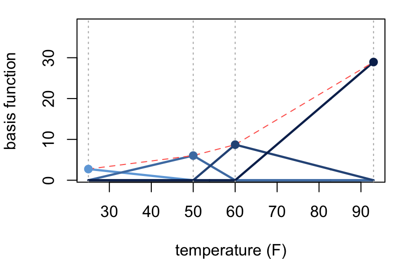
Local basis
The functions \(h_k(z) = p(z)^TE^{-1}\) define a local basis for piecewise linear functions.
For any piecewise linear \(f\) with knots at \(t_0, \dots, t_{K + 1}\)\[
f(x) = \sum_{k = 0}^{K + 1} c_k h_k(x)
\] for some coefficients \(c_0, \dots, c_{K + 1}\).
\(c_k = f(t_k)\) by construction
the slope on \([t_{k - 1}, t_k]\) is \[\frac{c_k - c_{k-1}}{t_k - t_{k-1}}\]
Drag a peak to change
ck, or a knot sideways.
c = t =
Revisiting ozone in LA
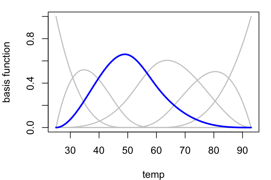
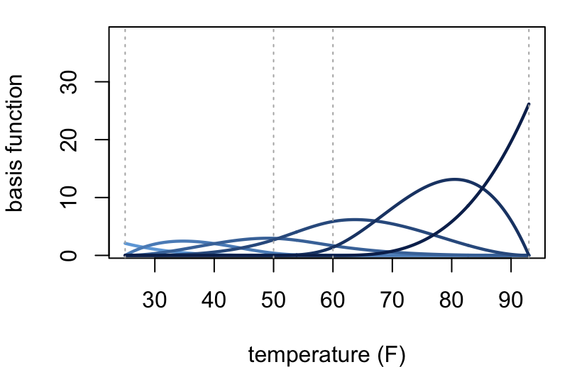
So instead of using pmax(...), specify a piecewise linear basis:
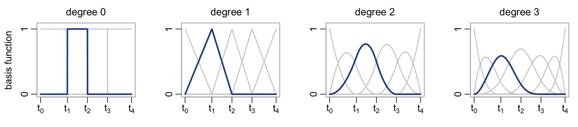
Repeating boundary knots to “clamp” bases gives \(k = 0, \dots, K + d\).
Each iteration defines a b-spline basis of degree \(d\).
General nonlinear relationships
Consider a general nonlinear regression model in one predictor:
\[
Y_i = f(x_i) + \epsilon_i
\]
Often one can approximate \(f\) by \[
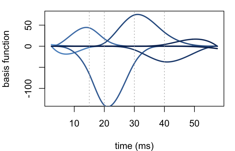
f(x) \approx \sum_{k = 0}^{K + d} c_k h_k^{(d)}(x)
\] where \(h_0^{(d)}, \dots, h_{K + d}^{(d)}\) is a b-spline basis.
Drag a peak to change
ck, or a knot sideways.
degree
The bs() function
Just as poly() generates polynomial terms, bs() generates basis expansions.
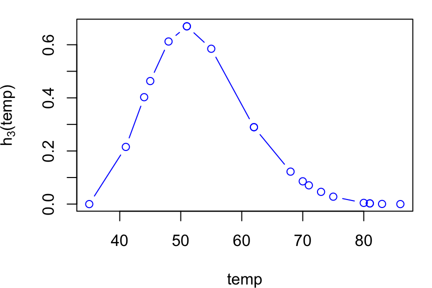
# downsample and sort for display purposestemp.sorted <-sample(ozone$temp, 20) |>sort()# compute basis expansiontemp.bs <-bs(temp.sorted, knots =c(50, 60), degree =3, intercept = T)# see structuretemp.bs[1:3, 1:5]
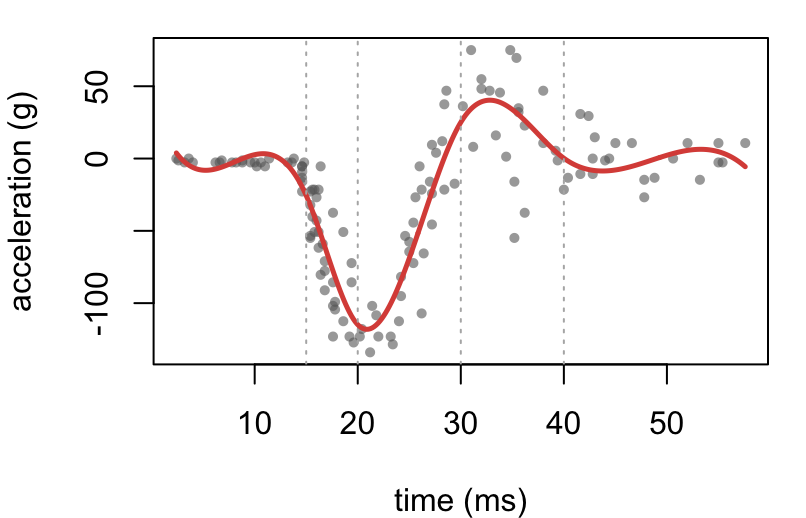
Nonlinear relationships can be estimated using a linear model for the basis expansion: \[
Y_i = \beta_0 h_0^{(d)}(x_i) + \beta_1 h_1^{(d)}(x_i) + \cdots + \beta_K h_{K+d}^{(d)}(x_i) + \epsilon_i
\]
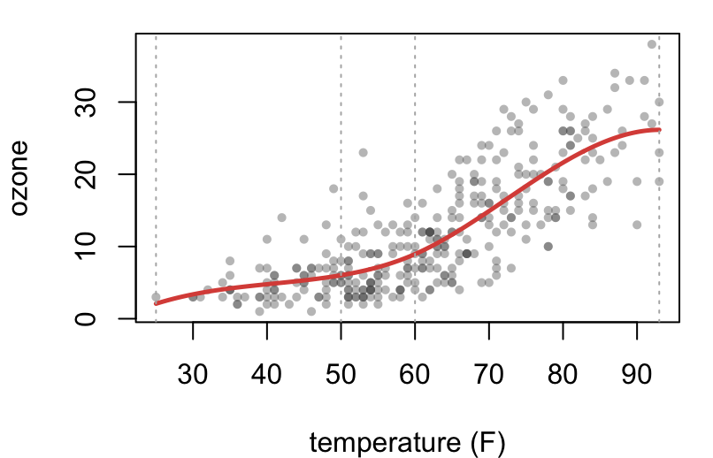
# fit a cubic spline modelH <-bs(ozone$temp, knots =c(50, 60), degree =3, intercept =TRUE)cub <-lm(O3 ~ H -1, data = ozone)summary(cub)$coef[, 1:2]