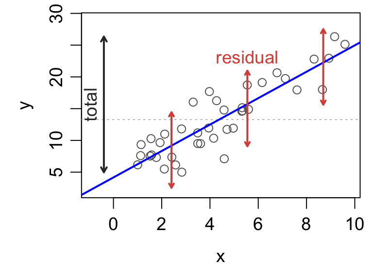
The standard measure of fit quality is the share of variation explained by the model: \[R^2 = \frac{SSR}{SST} = 1 - \frac{SSE}{SST}\]
Measuring model fit
Adding predictors always increases \(R^2\), even if modestly.
# update the model with a noise variableset.seed(92926)extra <-update(full, ~ . +rnorm(n =30, mean =0, sd =4))# compare r squaredc(original =summary(full)$r.squared, with.noise =summary(extra)$r.squared)
  original with.noise
 0.6517747  0.6540445
We can add an adjustment for the number of variables in the model \[
R^2_{\text{adj}} = 1 - \frac{SSE/(n-p)}{SST/(n-1)}
\]
# compare adjusted r squaredc(original =summary(full)$adj.r.squared, with.noise =summary(extra)$adj.r.squared)
  original with.noise
 0.6115948  0.5986917
So the model explains an estimated 61% of variation in taste scores.
The omnibus F test
Idea: test whether the model explains a significant amount of variation.
Suppose no predictor is associated with the response, i.e., \(H_0: \beta_1 = \cdots = \beta_{p-1} = 0\).
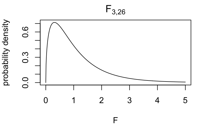
Under \(H_0\) and error normality, the relative share of variation explained by the model has a tractable sampling distribution: \[
F = \frac{n - p}{p - 1} \times \frac{SSR}{SSE} \sim F_{p-1,\,n-p}
\]
For the cheddar data the statistic is way out in the tail:
summary(full)$fstatistic
   value    numdf    dendf
16.22143  3.00000 26.00000
So the data provide evidence that the model explains a significant amount of variation.
That other stuff in the output
Check the bottom of the model summary for \(R^2\), adjusted \(R^2\), and the omnibus test.
summary(full)
Call:
lm(formula = taste ~ Acetic + H2S + Lactic, data = cheddar)

Residuals:
    Min      1Q  Median      3Q     Max
-17.390  -6.612  -1.009   4.908  25.449

Coefficients:
            Estimate Std. Error t value Pr(>|t|)
(Intercept) -28.8768    19.7354  -1.463  0.15540
Acetic        0.3277     4.4598   0.073  0.94198
H2S           3.9118     1.2484   3.133  0.00425 **
Lactic       19.6705     8.6291   2.280  0.03108 *
---
Signif. codes:  0 '***' 0.001 '**' 0.01 '*' 0.05 '.' 0.1 ' ' 1

Residual standard error: 10.13 on 26 degrees of freedom
Multiple R-squared:  0.6518,    Adjusted R-squared:  0.6116
F-statistic: 16.22 on 3 and 26 DF,  p-value: 3.81e-06
the data provide evidence that at least one compound is associated with taste
the compounds explain 61% of variance in taste scores
Another look at multicollinearity
Recall the car seat data: hipcenter on eight body measurements, for 38 drivers.
summary(seat)
Call:
lm(formula = hipcenter ~ ., data = seatpos)

Residuals:
    Min      1Q  Median      3Q     Max
-73.827 -22.833  -3.678  25.017  62.337

Coefficients:
             Estimate Std. Error t value Pr(>|t|)
(Intercept) 436.43213  166.57162   2.620   0.0138 *
Age           0.77572    0.57033   1.360   0.1843
Weight        0.02631    0.33097   0.080   0.9372
HtShoes      -2.69241    9.75304  -0.276   0.7845
Ht            0.60134   10.12987   0.059   0.9531
Seated        0.53375    3.76189   0.142   0.8882
Arm          -1.32807    3.90020  -0.341   0.7359
Thigh        -1.14312    2.66002  -0.430   0.6706
Leg          -6.43905    4.71386  -1.366   0.1824
---
Signif. codes:  0 '***' 0.001 '**' 0.01 '*' 0.05 '.' 0.1 ' ' 1

Residual standard error: 37.72 on 29 degrees of freedom
Multiple R-squared:  0.6866,    Adjusted R-squared:  0.6001
F-statistic:  7.94 on 8 and 29 DF,  p-value: 1.306e-05
Classic multicollinearity signature:
omnibus test is significant
but none of the partial tests are
So the fit says that some predictors matter but can’t identify which.
Perspectives on F tests
There are a few (equivalent) ways of looking at what’s being tested.
Coefficient values: is at least one coefficient in the set nonzero?
Recalling that \(SST = SSR_1 + SSE_1\) under \(\mathcal{M}_1\), we can rewrite the F statistic as \[
F = \frac{n-p}{p-1}\times\frac{SSR_1}{SSE_1}
= \frac{n-p}{p-1}\times\frac{SSE_0 - SSE_1}{SSE_1}
\]
It turns out that one can construct F tests to compare any nested models.
Nesting
\(\mathcal{M}_0\) is nested in \(\mathcal{M}_1\) if \(\mathcal{M}_0 \subseteq \mathcal{M}_1\). But what is model containment?
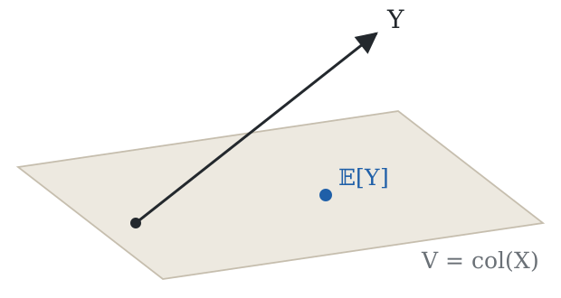
Formally, a model \(\mathcal{M}\) specifies that the mean lives in a subspace: \[
\mathbb{E}_\mathcal{M} [Y] \in V \subseteq \mathbb{R}^n
\]
In the general linear model one has \[
\mathbb{E}[Y] = X\beta \in \text{col}(X)
\]
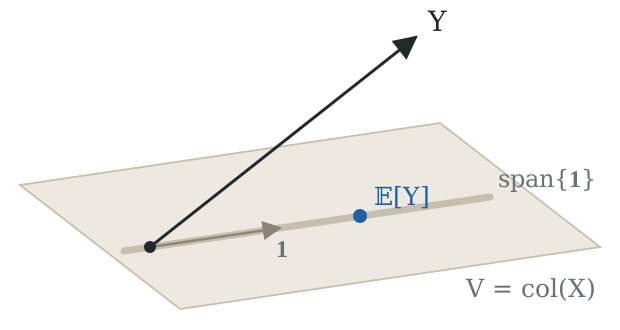
The intercept-only model is nested in the full model because \[
\text{span}\{\mathbf{1}\} \subseteq \text{col}(X)
\]
Geometry of the F test
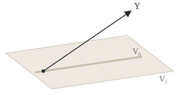
So for the omnibus F test we have
\[\begin{align*}
\mathcal{M}_0: Y &= \mathbf{1}\mu + \epsilon
\qquad&\text{null model} \\
\mathcal{M}_1: Y &= X\beta + \epsilon
\qquad&\text{full model} \\
\end{align*}\]
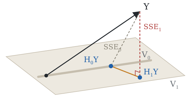
with the implied subspaces \(V_0 = \text{span}\{\mathbf{1}\}\) and \(V_1 = \text{col}(X)\).
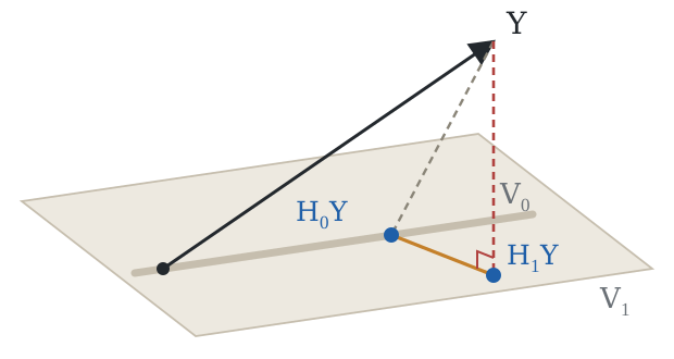
Least squares under each model gives the projections \[\begin{align*}
H_0 &= \frac{1}{n}\mathbf{1}\mathbf{1}^T\\
H_1 &= X(X^TX)^{-1}X^T
\end{align*}\]
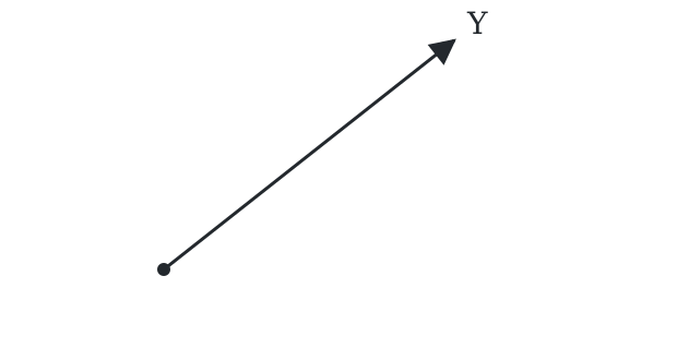
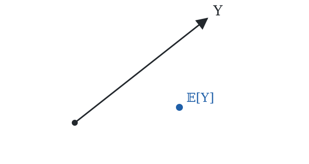
The error each model leaves behind is the distance from \(Y\) to its own subspace.
The geometry of the F test
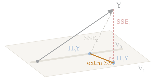
The “extra sum of squares” measures the distance between model fits.
So the F test is assessing whether the extra SS is large enough to support the full model: \[
F = \underbrace{\frac{SSE_0 - SSE_1}{SSE_1}}_\text{relative change in fit} \;\Big/\; \underbrace{\frac{\dim V_1 - \dim V_0}{n - \dim V_1}}_\text{relative change in df}
\]
Reconstructing the omnibus test
Revisiting the cheddar data, recall:
# f statisticsummary(full)$fstat
   value    numdf    dendf
16.22143  3.00000 26.00000
We can obtain this via a model comparison:
# full modelm1 <-lm(taste ~ ., data = cheddar)# reduced modelm0 <-lm(taste ~1, data = cheddar)# extra sum of squares F testanova(m0, m1)
Analysis of Variance Table

Model 1: taste ~ 1
Model 2: taste ~ Acetic + H2S + Lactic
  Res.Df    RSS Df Sum of Sq      F   Pr(>F)
1     29 7662.9
2     26 2668.4  3    4994.5 16.221 3.81e-06 ***
---
Signif. codes:  0 '***' 0.001 '**' 0.01 '*' 0.05 '.' 0.1 ' ' 1
In the ANOVA table:
Res.DF reports \(n - \text{dim}V\)
RSS reports \(SSE\)
Df reports the change in degrees of freedom
Sum of Sq reports the extra sum of squares
The extra sum of squares F test
The F test works for any nested models \(\mathcal{M}_0, \mathcal{M}_1\) for which \(V_0, V_1\) are linear subspaces.
\[
F = \underbrace{\frac{SSE_0 - SSE_1}{SSE_1}}_\text{relative change in fit} \;\Big/\; \underbrace{\frac{\dim V_1 - \dim V_0}{n - \dim V_1}}_\text{relative change in df}
\]