Applied Linear Models
STAT3530 Fall 2026
Recap
The simple linear model, in matrix form: \[Y = X\beta + \epsilon, \qquad \mathbb{E}[\epsilon] = 0, \qquad \text{Var}[\epsilon] = \sigma^2 I\] \[X = \left[\begin{array}{cc} 1 &x_1 \\ 1 &x_2 \\ \vdots &\vdots \\ 1 &x_n\end{array}\right]
\qquad\qquad
\beta = \left[\begin{array}{c} \beta_0 \\ \beta_1 \end{array}\right]\]
What we’ve covered:
estimation, inference, prediction, and interpretations
model diagnostics and transformations
leverage, outliers, and influential points
case studies and implementations in R
This model is called “simple” because there is only one explanatory variable.
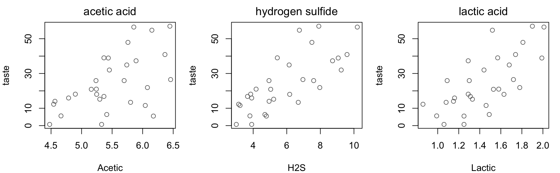
What explains the taste of cheddar?
Thirty mature cheeses, scored by a taste panel and assayed for three ripening compounds. Which compounds explain taste?
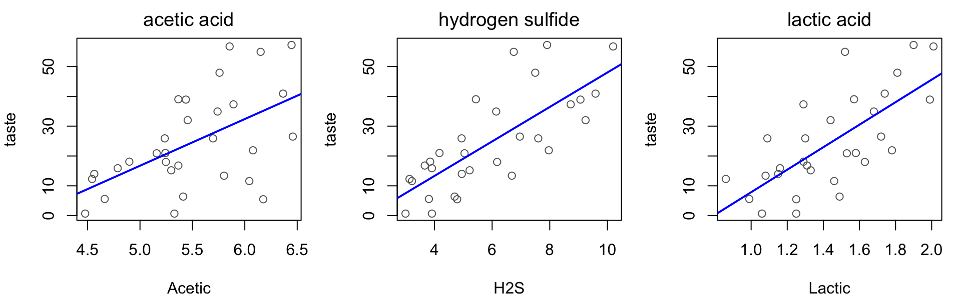
We could fit one model per predictor and check inference on the slope…
Acetic 15.65
4.496
3.481
0.0017
H2S 5.776
0.9458
6.107
0
Lactic 37.72
7.186
5.249
0
But…
we’d be using the data three times so tests aren’t independent
the predictors might be related
Predictor structure
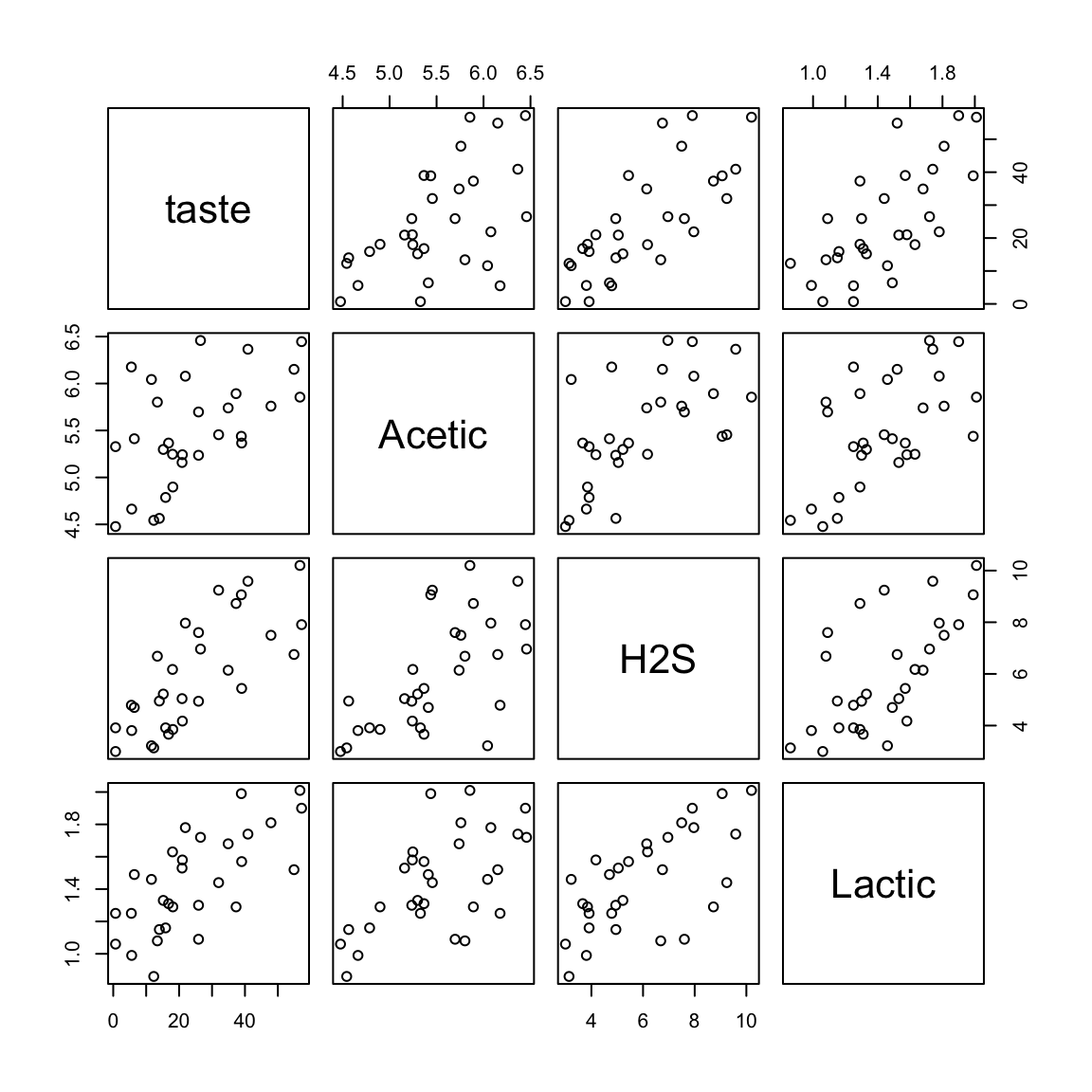
All three compounds track ripening, so the predictors are fairly correlated.
# all pairwise scatterplots pairs (cheddar)
# correlation matrix cor (cheddar) |> round (3 )
       taste Acetic   H2S Lactic
taste  1.000  0.550 0.756  0.704
Acetic 0.550  1.000 0.618  0.604
H2S    0.756  0.618 1.000  0.645
Lactic 0.704  0.604 0.645  1.000
Adjusting for one predictor
Modeling marginal relationships with taste ignores multivariate predictor structure.
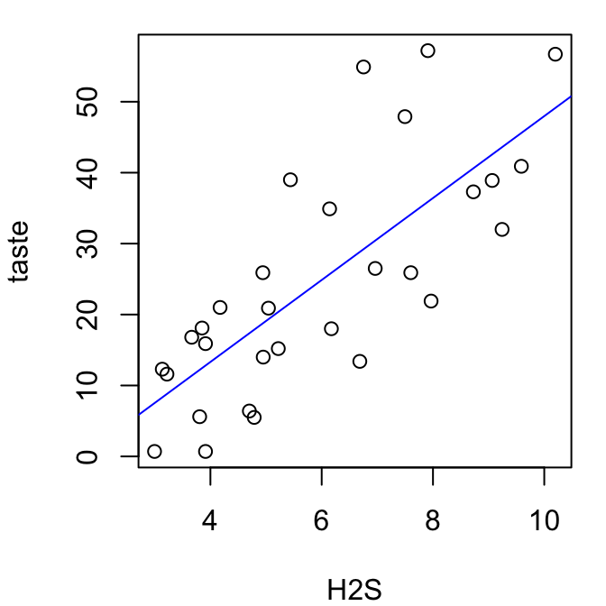
Consider first fitting the H2S model:
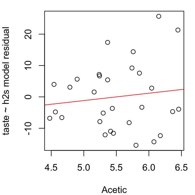
And then regressing residuals on Acetic acid:
Before, the marginal p -value for the slope in the Acetic variable was 0.0017
But in the residual model, the p -value is 0.507
So the association vanishes if we adjust for H2S. How do we model this?
More columns in \(X\)
What if we write the same model \(Y = X\beta + \epsilon\) but include more predictors, like so:
\[X = \left[\begin{array}{cccc}
1 &x_{11} &x_{12} &x_{13} \\
1 &x_{21} &x_{22} &x_{23} \\
\vdots &\vdots &\vdots &\vdots \\
1 &x_{n1} &x_{n2} &x_{n3}
\end{array}\right]
\qquad
\beta = \left[\begin{array}{c} \beta_0 \\ \beta_1 \\ \beta_2 \\ \beta_3\end{array}\right]\]
Dimensions change:
\(X\) is \(n \times 4\) \(\beta\) is \(4 \times 1\) entries.
Estimation and inference does not:
none of the previous arguments from weeks 1-5 depend on the dimension of \(X\)
only that, whatever its dimension, it is full rank
Fitting the multiple predictor model
# fit the multiple regression model <- lm (taste ~ Acetic + H2S + Lactic, data = cheddar)summary (fit)$ coefficients
               Estimate Std. Error    t value    Pr(>|t|)
(Intercept) -28.8767696  19.735418 -1.4631952 0.155399149
Acetic        0.3277413   4.459757  0.0734886 0.941979774
H2S           3.9118411   1.248430  3.1334077 0.004247081
Lactic       19.6705434   8.629055  2.2795710 0.031079481
This corresponds to the fitted model equation:
\[
\mathbb{E}[\text{taste}] = -28.88 + 0.33\,\text{Acetic} + 3.91\,\text{H2S} + 19.67\,\text{Lactic}
\]
Notice Acetic is no longer significant. But what do the coefficients mean?
Coefficient interpretations
Our model now gives:
\[
\mathbb{E}[\text{taste}] = \beta_0 + \beta_1\,\text{Acetic} + \beta_2\,\text{H2S} + \beta_3\,\text{Lactic}
\]
So for the increment \(\text{Lactic} \to \text{Lactic} + 1\) , we get:
\[\begin{align*}
\mathbb{E}[\text{taste}] &= \color{grey}{\beta_0 + \beta_1\,\text{Acetic} + \beta_2\,\text{H2S}} + \beta_3\,(\text{Lactic} + 1)\\
&= \color{grey}{\beta_0 + \beta_1\,\text{Acetic} + \beta_2\,\text{H2S}} + \beta_3\,\text{Lactic} + \beta_3 \\
&= \color{grey}{\beta_0 + \beta_1\,\text{Acetic} + \beta_2\,\text{H2S} + \beta_3\,\text{Lactic}} + \beta_3\\
\end{align*}\]
So \(\beta_3\) is the change in mean taste per unit increase in lactic acid concentration…
…if acetic acid and H2S concentrations are held constant
The general linear model
For the general linear model with \(p - 1\) predictors, \(Y = X\beta + \epsilon\) becomes \[
\left[\begin{array}{c} Y_1 \\Y_2 \\\vdots \\Y_n \end{array}\right]
= \left[\begin{array}{cccc}
1 &x_{11} &\cdots &x_{1\,p-1} \\
1 &x_{21} &\cdots &x_{2\,p-1} \\
\vdots &\vdots &\ddots &\vdots \\
1 &x_{n1} &x_{n2} &x_{n\,p-1}
\end{array}\right]
\left[\begin{array}{c} \beta_0 \\ \beta_1 \\ \vdots \\ \beta_{p-1}\end{array}\right]
+ \left[\begin{array}{c} \epsilon_1 \\ \epsilon_2 \\ \vdots \\ \epsilon_{n}\end{array}\right]
\]
where assumptions are unchanged:
(linearity) \(\mathbb{E}[\epsilon] = 0\)
(constant variance) \(\text{var}[\epsilon] = \sigma^2 I\)
(independence) \(\epsilon_i \perp \epsilon_j\)
(normality) \(\epsilon \sim \mathcal{N}(0, \sigma^2 I)\)
And \(Y, \epsilon\) remain \(n \times 1\) but now:
\(X\) is \(n\times p\) \(\beta\) is \(p\times 1\)
Thus, simple linear regression was the special case with \(p = 2\) .
Estimation and inference
All the earlier arguments go through unchanged:
least squares minimizes \(SSE(\beta) = \|Y - X\beta\|^2\)
the least squares estimator is still \(\hat\beta = (X^TX)^{-1}X^TY\) and has all the same properties
the hat matrix \(H = X(X^TX)^{-1}X^T\) still has all the same properties
the geometry is unchanged
under error normality we still have \(\hat\beta \sim N(\beta, \sigma^2(X^TX)^{-1})\)
So inference on the coefficients is given by:
\[
T_j = \frac{\hat\beta_j - \beta_j}{\text{SE}(\hat\beta_j)} \sim t_{n - p}
\]
Only now, the coefficient \(\beta_j\) is the change in mean response per increment in \(x_j\) after accounting for all other variables in the model.
What explains the taste of cheddar?
# fit the multiple regression model <- lm (taste ~ Acetic + H2S + Lactic, data = cheddar)# coefficient summary table summary (fit)$ coefficients
               Estimate Std. Error    t value    Pr(>|t|)
(Intercept) -28.8767696  19.735418 -1.4631952 0.155399149
Acetic        0.3277413   4.459757  0.0734886 0.941979774
H2S           3.9118411   1.248430  3.1334077 0.004247081
Lactic       19.6705434   8.629055  2.2795710 0.031079481
# confidence intervals confint (fit)
                 2.5 %    97.5 %
(Intercept) -69.443503 11.689964
Acetic       -8.839420  9.494902
H2S           1.345656  6.478026
Lactic        1.933267 37.407820
Now we can answer the question.
adjusted for other compounds, H2S and lactic acid are significantly associated with taste
acetic acid is not
Moreover, with 95% confidence,
each increment in H2S is associated with an estimated increase in mean taste score between 1.35 and 6.48 points
each increment in lactic acid is associated with an estimated increase in mean taste score between 1.93 and 37.41 points
Standardizing for interpretation
Predictor scales are not comparable, so relative practical significance is difficult to assess.
Centering and scaling will do the trick:
\[
x_j \leftarrow \frac{x_j - \bar{x}_j}{s_j}
\]
# refit after standardization <- lm (taste ~ scale (Acetic) + scale (H2S) + scale (Lactic), data = cheddar)summary (refit)$ coefficients
                Estimate Std. Error    t value     Pr(>|t|)
(Intercept)   24.5333333   1.849605 13.2640910 4.413822e-13
scale(Acetic)  0.1871004   2.545979  0.0734886 9.419798e-01
scale(H2S)     8.3200133   2.655260  3.1334077 4.247081e-03
scale(Lactic)  5.9698141   2.618832  2.2795710 3.107948e-02
A one unit increase is now a one SD increase, so H2S is associated with a relatively larger change in mean taste than lactic acid, but they are of comparable importance.
# confidence intervals confint (refit)
                   2.5 %    97.5 %
(Intercept)   20.7314151 28.335252
scale(Acetic) -5.0462334  5.420434
scale(H2S)     2.8620474 13.777979
scale(Lactic)  0.5867273 11.352901
+1 SD changes in predictors are associated with changes of…
2.86 to 13.78 points for H2S
0.59 to 11.35 points for lactic acid
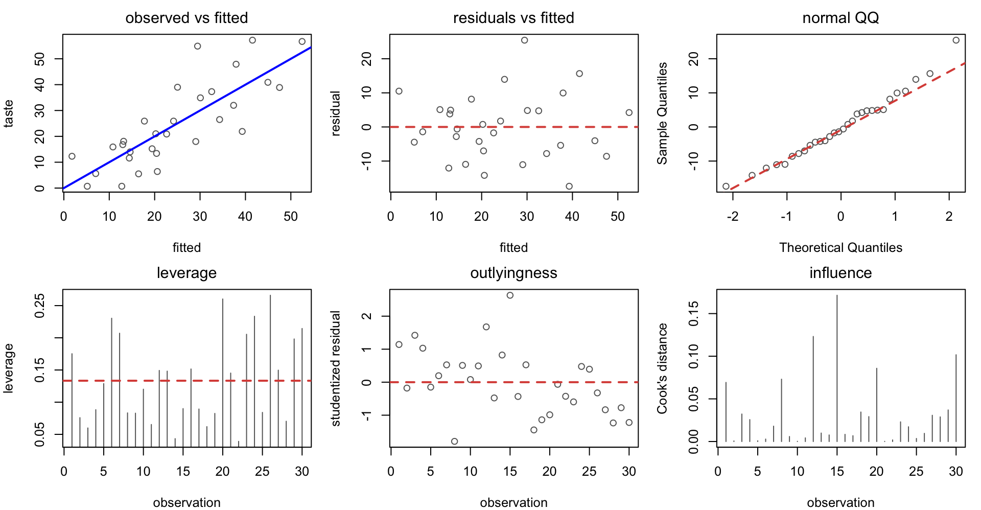
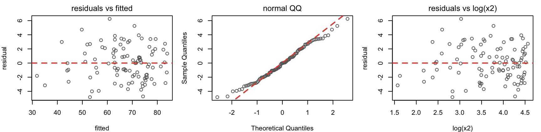
Diagnostics: the same plots
No issues anywhere for this model.
What if you had spotted an issue?
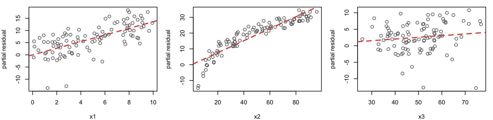
Here is a model fit to data simulated from
\[
Y = \beta_0 + \beta_1 x_1 + \beta_2 \log(x_2) + \beta_3 x_3 + \epsilon
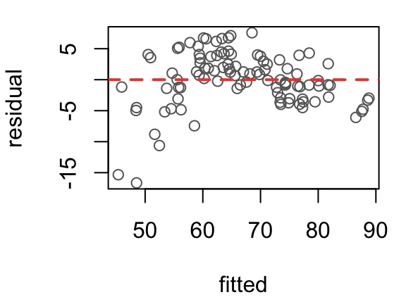
\] But the model is misspecified
<- lm (y ~ x1 + x2 + x3, data = sim3)
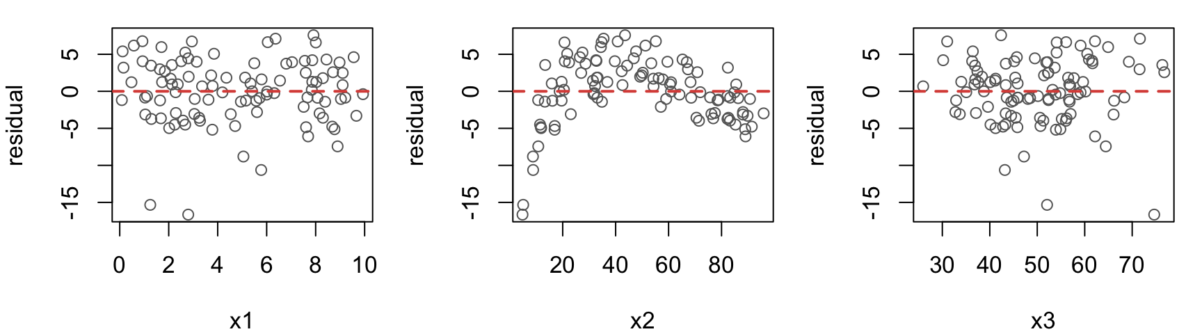
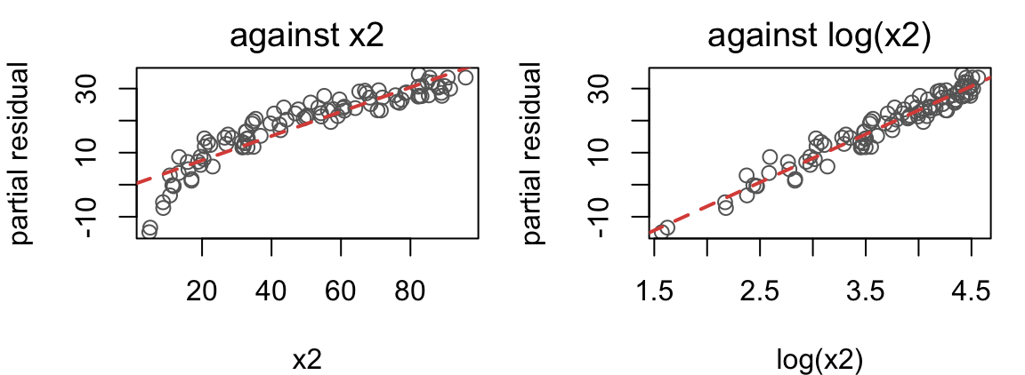
Plot residuals against each predictor individually to spot the issue: x2.
Fixing model specification
How should we adjust x2?
Take what the model could not explain and add back one predictor’s fitted contribution:
\[e_j = e + \hat\beta_j x_j\]
This is called a partial residual ; plots of \(e_j\) against \(x_j\) show the relationship after adjusting (linearly) for other variables.
x2 traces a logarithm — steep, then flattening — so that is the fix.
The corrected model
<- lm (y ~ x1 + log (x2) + x3, data = sim3)summary (better)$ coefficients
               Estimate Std. Error    t value     Pr(>|t|)
(Intercept)  0.92417884 1.82191177  0.5072577 6.131373e-01
x1           1.15383750 0.08595770 13.4233168 9.364092e-24
log(x2)     15.01377350 0.34633218 43.3507892 7.568222e-65
x3           0.09746968 0.02244789  4.3420414 3.499016e-05
Clean, and \(R^2\) rises from \(0.85\) to \(0.95\) .
Visualizing the model
With \(p = 3\) we are fitting a 2D plane in 3D space.
Drag a corner to tilt the plane; drag the background to rotate.
β̂0 = 1 = (H2S) 2 = (lactic)
least squares
flat
For \(p > 3\) we would be fitting a \((p-1)\) -dimensional hyperplane in \(p\) -dimensional space.
But we are still projecting from \(\mathbb{R}^n\) into \(\mathbb{R}^p\) .
Predicting the taste of new cheeses
As before, given new \(x_0\) , the prediction is \(\hat{Y} = x_0 \hat\beta\) .
<- data.frame (Acetic = c (5.0 , 6.2 ), H2S = c (4.0 , 9.0 ), Lactic = c (1.2 , 1.8 ))
Here the new data are \[
x_0 = \left[\begin{array}{cccc}
1 & 5.0 & 4.0 & 1.2 \\
1 & 6.2 & 9.0 & 1.8
\end{array}\right]
\]
predict (full, new, interval = 'confidence' )
       fit       lwr      upr
1 12.01395  6.578536 17.44937
2 43.76877 36.786956 50.75059
predict (full, new, interval = 'prediction' )
       fit       lwr     upr
1 12.01395 -9.507692 33.5356
2 43.76877 21.805549 65.7320
And as before, the confidence and prediction intervals use different standard errors:
(confidence) \(SE(\hat{Y}) = \hat\sigma \sqrt{x_0^T (X^T X)^{-1} x_0}\)
(prediction) \(SE(\hat{Y}_{\text{pred}}) = \hat\sigma\sqrt{1 + x_0^T (X^T X)^{-1} x_0}\)
A new failure mode
Recall that \(X\) must be full rank; otherwise \(X^TX\) is singular and \(\hat\beta\) can’t be computed.
Full rank for \(X_{n\times p}\) requires columns are linearly independent and \(n > p\) .
Here’s an example that breaks this: \[
X = \left[\begin{array}{ccccc}
1 &x_1 &x_2 &x_3 &2x_3
\end{array}\right]
\] since \(x_4\) is a rescaled copy of \(x_3\) .
And here’s what happens if you try and fit that
<- cheddar$ Lactic2 <- 2 * cheddar2$ Lacticlm (taste ~ ., data = cheddar2)
Call:
lm(formula = taste ~ ., data = cheddar2)

Coefficients:
(Intercept)       Acetic          H2S       Lactic      Lactic2
   -28.8768       0.3277       3.9118      19.6705           NA
Multicollinearity
Usually predictors aren’t exactly linearly dependent but instead get close — sometimes variables measure similar information.
For example, suppose we measured a new compound that tracks lactic acid very closely:
<- cheddar$ Schmactic <- cheddar$ Lactic + rnorm (n = 30 , mean = 0 , sd = 0.05 )cor (cheddar2[, - 1 ])
             Acetic       H2S    Lactic Schmactic
Acetic    1.0000000 0.6179559 0.6037826 0.6030751
H2S       0.6179559 1.0000000 0.6448123 0.6463599
Lactic    0.6037826 0.6448123 1.0000000 0.9840876
Schmactic 0.6030751 0.6463599 0.9840876 1.0000000
Now the model can still be fit, but \(X^TX\) is close to singular
<- lm (taste ~ ., data = cheddar2) summary (fit.multi)$ coefficients
               Estimate Std. Error     t value    Pr(>|t|)
(Intercept) -29.4318174  20.025787 -1.46969594 0.154117545
Acetic        0.4105821   4.522246  0.09079162 0.928381711
H2S           3.9604812   1.268224  3.12285575 0.004486276
Lactic       38.9224085  35.478086  1.09708311 0.283060329
Schmactic   -19.4524634  34.741612 -0.55991828 0.580518095
so the model can’t distinguish between lactic and schmactic.
This is called multicollinearity .
Multicollinearity, conceptually
Consider \(p = 3\) . If the two predictors are correlated and \(x_1 \approx a\,x_2 + b\) , then the model approaches \[
\mathbb{E}[Y] \approx \beta_0 + \beta_1 x_1 + \beta_2 (a\,x_1 + b) = (\beta_0 + \beta_2 b) + (\beta_1 + \beta_2 a) x_1
\] so since \(a, b\) are unknown, different combinations of \(\beta_1, \beta_2\) give similar specifications.
This happens whenever two predictors are providing duplicate signal.
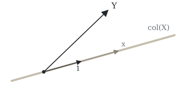
Multicollinearity, geometrically
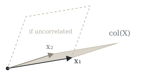
Exact collinearity in SLR: \(x = c\mathbf{1}\) , and \(col(X)\) is only a line.
Near collinearity: \(col(X)\) is still a plane, but a very thin one.
Either way the projection \(\hat{Y}\) is fine; it’s the coordinates \(\hat{\beta}\) that suffer.
Multicollinearity, mathematically
Under the hood, what happens is that \(\text{det}(X^TX)\) is driven toward zero
<- model.matrix (full) # without schmactic <- model.matrix (fit.multi) # with c (original = det (t (X0) %*% X0), schmactic = det (t (X) %*% X))
 original schmactic
31690.066  2767.729
So the entries of \((X^T X)^{-1}\) blow up
            (Intercept)      Acetic         H2S       Lactic    Schmactic
(Intercept)  3.80433519 -0.76119163  0.08648892  -0.39478025   0.32670462
Acetic      -0.76119163  0.19400281 -0.02023451  -0.07985509  -0.04876061
H2S          0.08648892 -0.02023451  0.01525779  -0.01717048  -0.02862987
Lactic      -0.39478025 -0.07985509 -0.01717048  11.94042991 -11.33176958
Schmactic    0.32670462 -0.04876061 -0.02862987 -11.33176958  11.44984298
And you get high uncertainty around similar predictors.
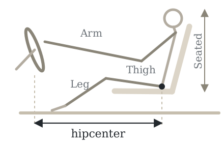
Car seat position
Where a driver sets the seat: hipcenter is the distance from the steering wheel to the hip, and the predictors are eight measurements of the driver.
Example
Car seat position: hipcenter is how far a driver’s hips sit from the steering wheel, with eight body measurements, for 38 drivers.
<- faraway:: seatpos<- lm (hipcenter ~ ., data = seatpos)round (summary (seat)$ coefficients, 3 )
            Estimate Std. Error t value Pr(>|t|)
(Intercept)  436.432    166.572   2.620    0.014
Age            0.776      0.570   1.360    0.184
Weight         0.026      0.331   0.080    0.937
HtShoes       -2.692      9.753  -0.276    0.784
Ht             0.601     10.130   0.059    0.953
Seated         0.534      3.762   0.142    0.888
Arm           -1.328      3.900  -0.341    0.736
Thigh         -1.143      2.660  -0.430    0.671
Leg           -6.439      4.714  -1.366    0.182
Every measurement tracks body size:
cor (seatpos$ Ht, seatpos$ HtShoes)
c (residual = sigma (seat), total = sd (seatpos$ hipcenter))
residual    total
37.72029 59.64738
The model reduces variation yet nothing is significant.
This is correct behavior, since the model can’t be expected to distinguish signal among a set of very similar predictors.
Data analysis activity
In 1971 a sample of Canadians rated 102 occupations for prestige. The data pair those ratings with the average education , average income , and percentage women in each occupation.
Which of the three are associated with prestige, and how much is each worth?
look at the data with pairs()
fit a model and read summary()
check the diagnostics, one residual plot per predictor
check the partial residual plots; refit if a predictor is on the wrong scale
report confidence intervals and answer the question
scripts/09-multiple-regression.R walks through the same five steps on the cheddar data first.
Is the model any good?
Two ways to understand this.
Prediction: does the model perform well out of sample?
Explanation: does the model describe the current sample well?
They aren’t mutually exclusive, but they are different goals.
Understanding prediction error
A natural measurement is mean square prediction error . For a single observation \(Y_0\) this decomposes as
\[
\mathbb{E}\left[(Y_0 - \hat{Y}_0)^2\right]
= \underbrace{\text{var}(Y_0)}_{\sigma^2} + \underbrace{\text{var}(\hat{Y}_0)}_\text{variance} - \underbrace{2\,\text{cov}(Y_0, \hat{Y}_0)}_\text{covariance} + \underbrace{(\mathbb{E}[Y_0] - \mathbb{E}[\hat{Y}_0])^2}_\text{bias}
\]
For the linear model, \(\hat{Y}_0 = x_0^T\hat\beta\) is a function of some data \(Y\) .
The bias term depends on whether
\(Y_0\) follows the same data generating process as \(Y\) the model is correctly specified
The covariance term depends on whether \(Y_0\) is included in \(Y\) (“in sample”):
if not, \(\text{cov}(Y_0, \hat{Y}_0) = 0\)
if so, \(\text{cov}(Y_0, \hat{Y}_0) = \sigma^2 h_{00} > 0\)
In sample versus out of sample
The basic distinction: was \(Y_0\) part of the sample you used to fit the model?
Let’s suppose for simplicity that \(x_0\) is included either way.
\[
\mathbb{E}\left[(Y_0 - \hat{Y}_0)^2\right]
= \underbrace{\text{var}(Y_0)}_{\sigma^2} + \underbrace{\text{var}(\hat{Y}_0)}_\text{variance} - \underbrace{2\,\text{cov}(Y_0, \hat{Y}_0)}_\text{covariance} + \underbrace{(\mathbb{E}[Y_0] - \mathbb{E}[\hat{Y}_0])^2}_\text{bias}
\]
If the data generating process is unchanging and the model is correctly specified:
\[
\mathbb{E}\left[(Y_0 - \hat{Y}_0)^2\right]
= \begin{cases}
\sigma^2 + \sigma^2 h_{00} - 2\sigma^2 h_{00}
&= \sigma^2 (1 - h_{00}) &\,,\;\text{in sample}\\
\sigma^2 + \sigma^2 h_{00}
&= \sigma^2 (1 + h_{00}) &\,,\;\text{out of sample}\\
\end{cases}
\]
So leverage diminishes the in-sample MSPE relative to “genuine” new data.
Measuring prediction error
To estimate mean square prediction error, take an average
\[
\frac1n \sum_{i = 1}^n (Y_i - \hat{Y}_i)^2
\]
But compare what happens in-sample and out-of-sample:
# in sample: every cheese helped fit the model that predicts it mean (resid (full)^ 2 )# out of sample: predict each cheese from a model fit without it <- sapply (1 : 30 , function (i)predict (lm (taste ~ ., data = cheddar[- i, ]), cheddar[i, ]))mean ((cheddar$ taste - loo)^ 2 )
Clever trick: no refitting needed, since \(Y_i - \hat{Y}_{i(i)} = \frac{e_i}{1 - h_{ii}}\)
mean ((resid (full) / (1 - hatvalues (full)))^ 2 )
How good is the model (prediction)?
So our first answer is that for the cheddar data:
# out of sample mspe <- mean ((resid (full) / (1 - hatvalues (full)))^ 2 )
But what does this mean exactly?
It’s variance-like, so take a square root and interpret:
# square root <- sqrt (mspe)
So we can predict taste scores to within ten points on average.