Applied Linear Models
STAT3530 Fall 2026
Log-transforming the response
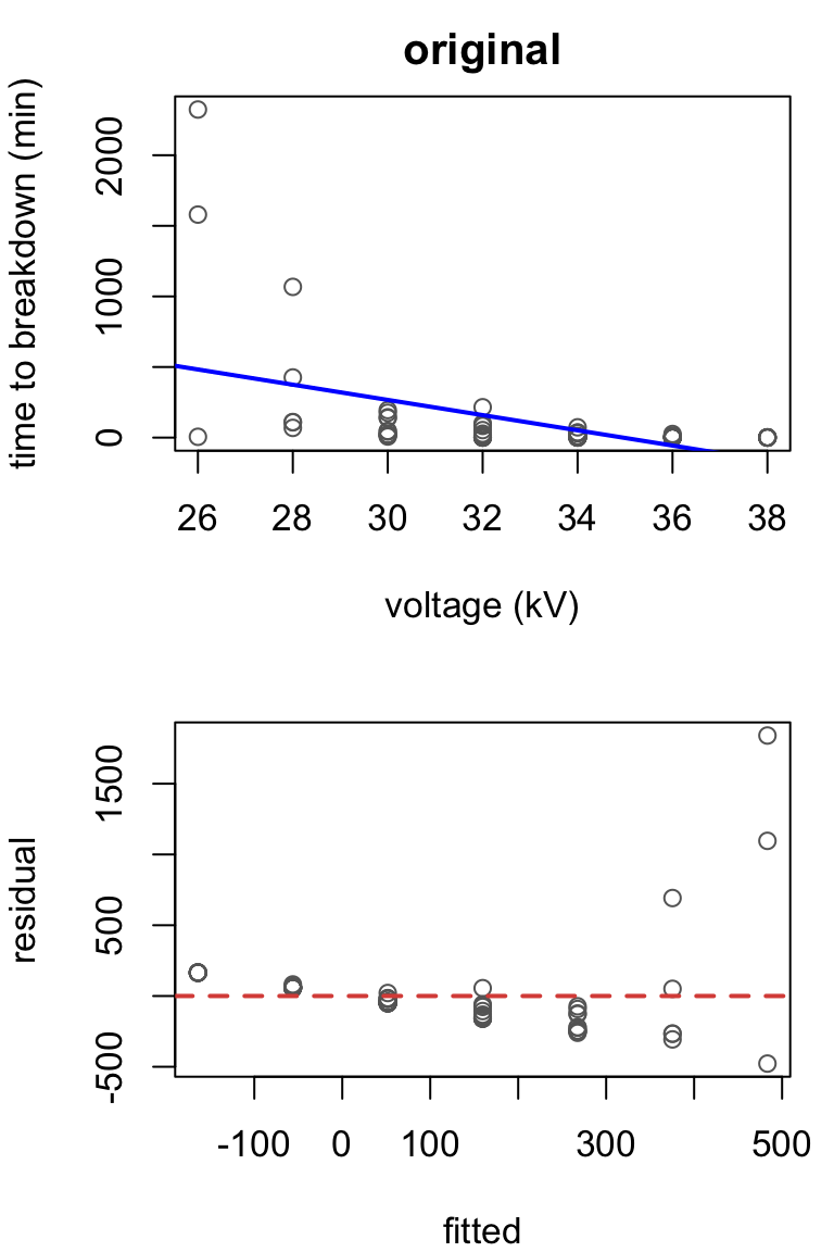
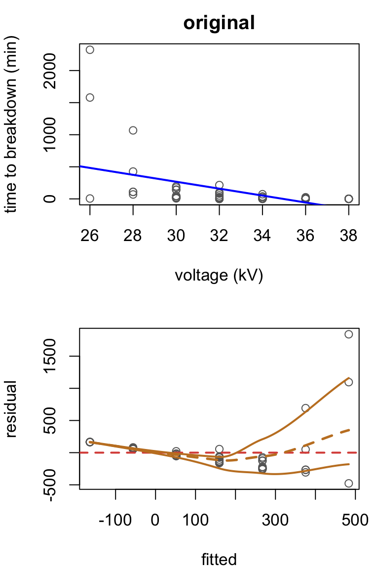
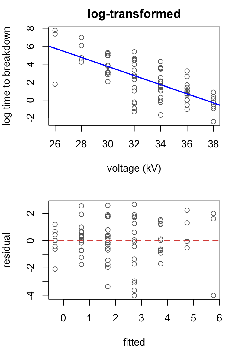
Time until an electrical insulating fluid breaks down, for 76 samples tested at seven voltages.
Original: \[Y_i = \beta_0 + \beta_1 x_i + \epsilon_i\]
Issue: nonconstant variance, curvature.
Transformation: \[\log(Y_i) = \beta_0 + \beta_1 x_i + \epsilon_i\] The curve is gone; variance isn’t perfect, but much better.
Back-transformation
              Estimate Std. Error   t value     Pr(>|t|)
(Intercept) 18.9554587 1.91001876  9.924226 3.052326e-15
voltage     -0.5073649 0.05739595 -8.839734 3.340072e-13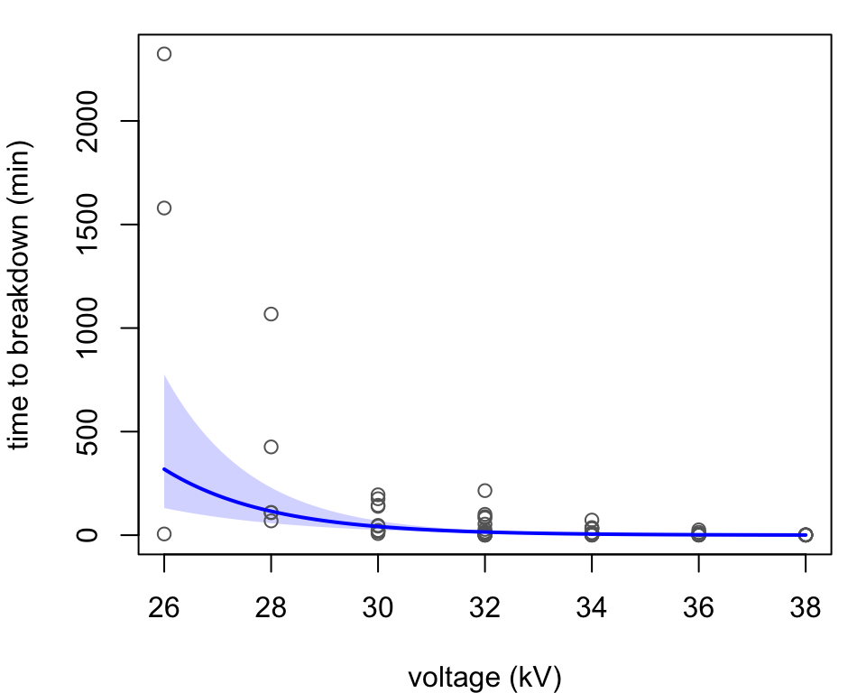
Fitted model: \[\hat{Y}_i = e^{18.96}\, e^{-0.507\, x_i}\]
Here, \(\hat{Y}_i\) estimates the median breakdown time.
Each additional kV multiplies \(\hat{Y}\) by a factor of \(e^{-0.507} = 0.60\).
Each additional kV is associated with an estimated 40% decrease in median breakdown time.
Log-transforming the predictor
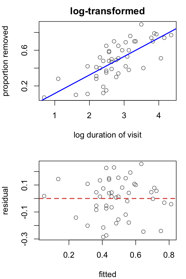
Proportion of a lily’s pollen removed by a bee, against how long the bee’s visit lasted, for 47 visits.
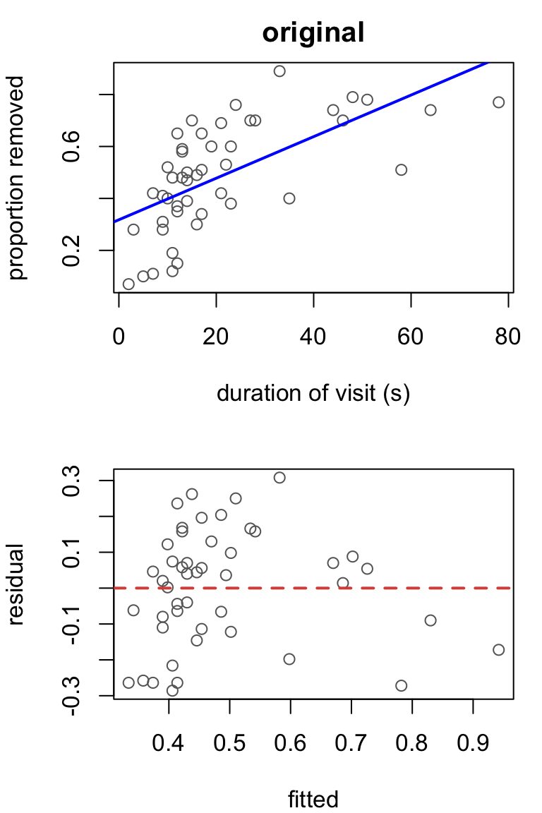
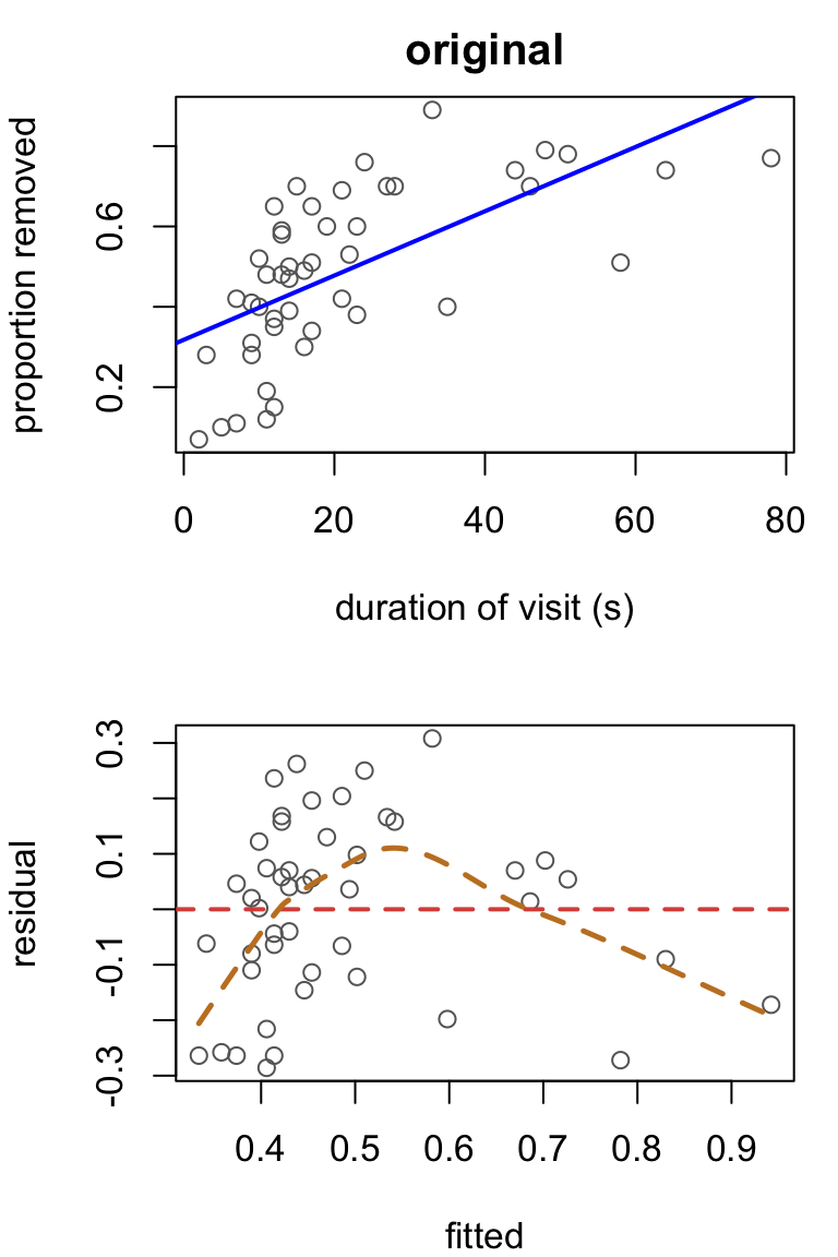
Original model: \[Y_i = \beta_0 + \beta_1 x_i + \epsilon_i\]
Issue: curvature.
Transformation: \[Y_i = \beta_0 + \beta_1 \log(x_i) + \epsilon_i\] The curve is gone. The spread was never the problem, so the response is left alone.
Back-transformation
                 Estimate Std. Error   t value     Pr(>|t|)
(Intercept)   -0.09221658 0.08149970 -1.131496 2.638404e-01
log(duration)  0.20760092 0.02822562  7.355052 3.040327e-09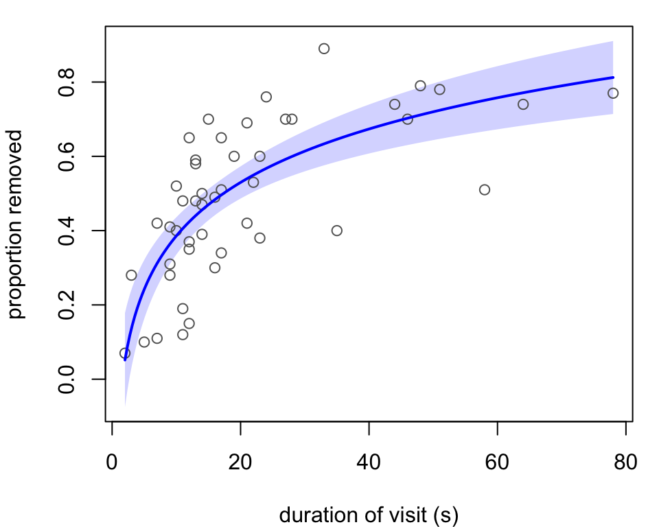
Fitted model: \[\hat{Y}_i = -0.092 + 0.208 \log(x_i)\]
\(\hat{Y}_i\) still estimates the mean proportion of pollen removed.
Doubling the length of a visit adds \(0.208 \log 2 = 0.144\) to \(\hat{Y}\).
Each doubling of visit length is associated with an estimated 14 percentage point increase in the mean proportion of pollen removed.
Log-transforming both
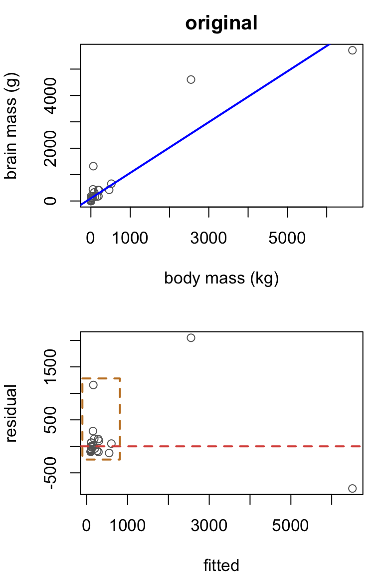
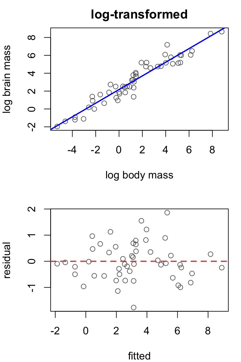
Brain mass against body mass for 51 species of mammal.
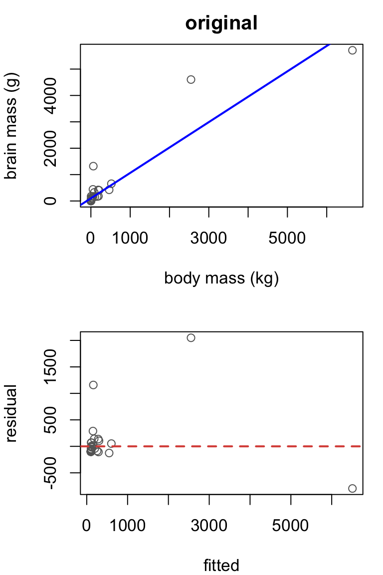
Original model: \[Y_i = \beta_0 + \beta_1 x_i + \epsilon_i\]
Issue: model is obviously not on the right scale.
Transformation: \[\log(Y_i) = \beta_0 + \beta_1 \log(x_i) + \epsilon_i\] Often you’d find this sequentially by first transforming \(x\), then transforming \(Y\).
Back-transformation
             Estimate Std. Error  t value     Pr(>|t|)
(Intercept) 2.1737368 0.11018768 19.72758 5.870654e-25
log(body)   0.7636132 0.03234614 23.60755 2.022309e-28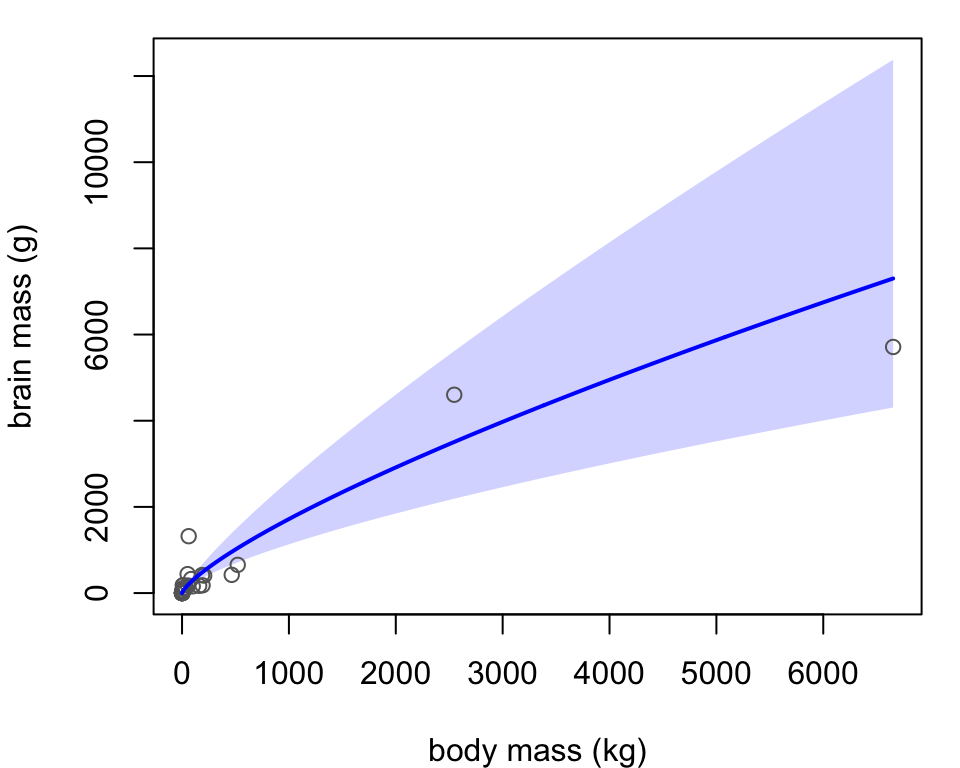
Fitted model: \[\hat{Y}_i = e^{2.17}\, x_i^{0.764}\]
Here, \(\hat{Y}_i\) estimates the median brain mass.
Doubling body mass multiplies \(\hat{Y}\) by a factor of \(2^{0.764} = 1.70\).
Each doubling of body mass is associated with an estimated 70% increase in median brain mass.
Square root of the response
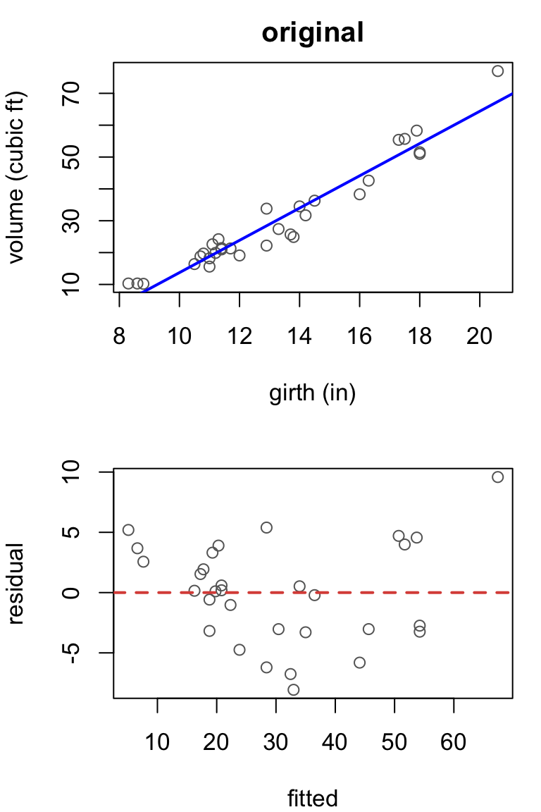
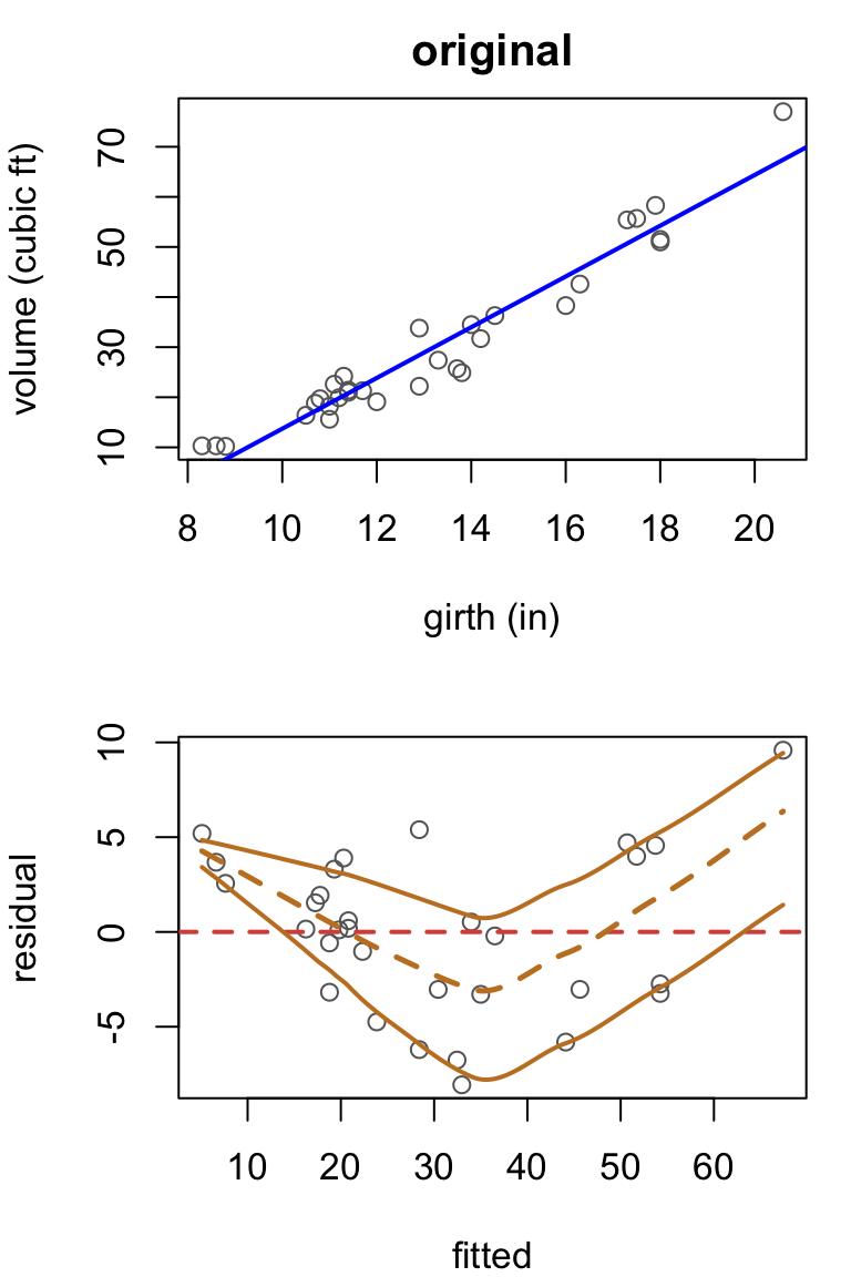
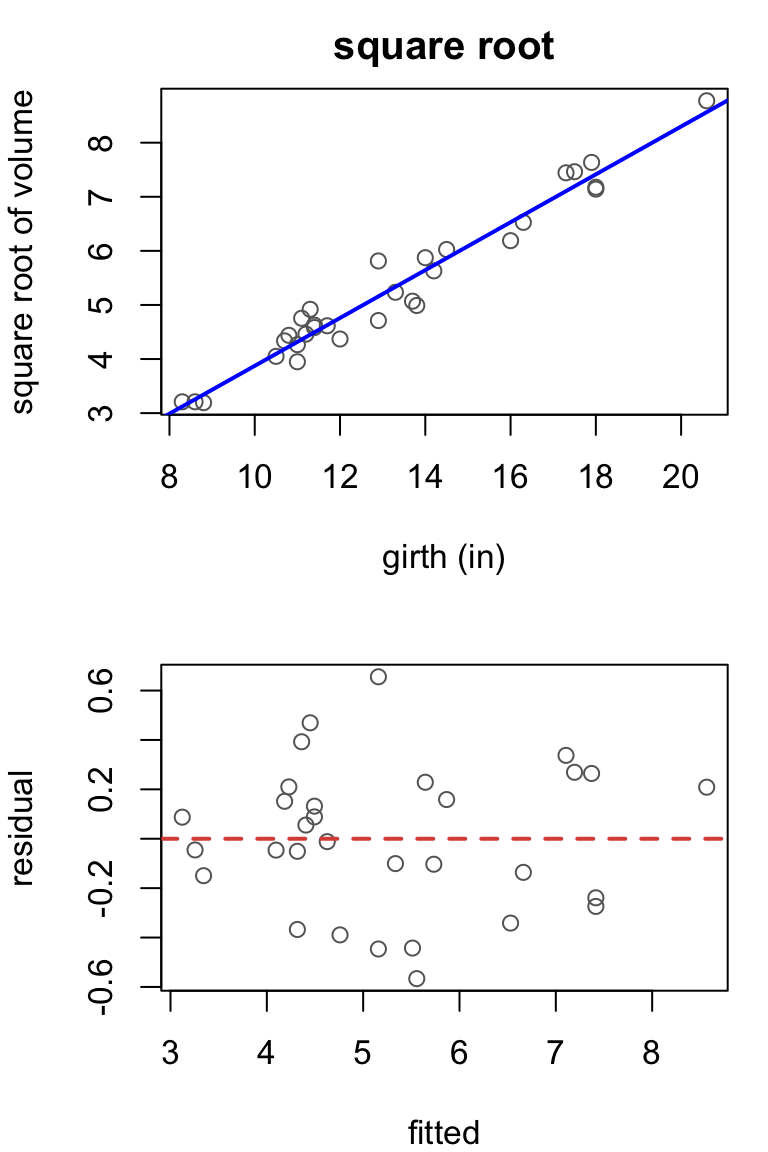
Timber volume against trunk girth for 31 black cherry trees. Volume grows roughly with girth squared, so its square root should grow roughly in a straight line.
Original model: \[Y_i = \beta_0 + \beta_1 x_i + \epsilon_i\]
Issue: nonlinearity, and some nonconstant variance.
Transformation: \[\sqrt{Y_i} = \beta_0 + \beta_1 x_i + \epsilon_i\] The curve and the fan are both largely gone.
Back-transformation
              Estimate Std. Error   t value     Pr(>|t|)
(Intercept) -0.5518275 0.23718993 -2.326522 2.718265e-02
Girth        0.4426244 0.01743619 25.385381 2.347333e-21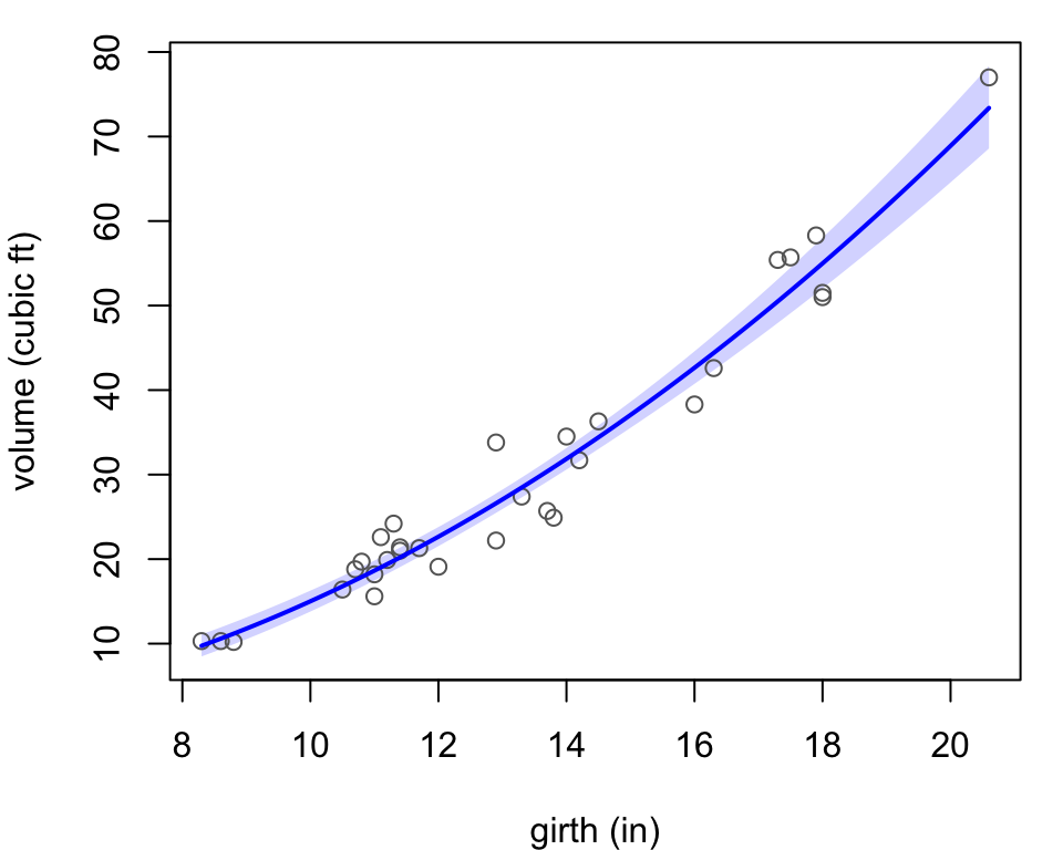
Fitted model: \[\hat{Y}_i = \left(-0.552 + 0.443\, x_i\right)^2\]
Here, \(\hat{Y}_i\) estimates the median volume.
The change in \(\hat{Y}\) from an extra inch of girth depends on starting size.
An extra inch of girth is associated with an estimated increase in median volume of about 3.6 cubic feet for a 10 inch tree, and 6.8 cubic feet for an 18 inch tree.
Reciprocal of the response
City fuel economy against weight for 93 car models on sale in the US in 1993.
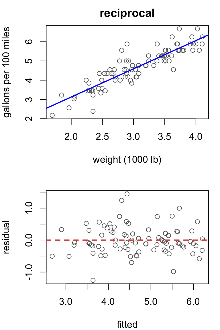
Fuel economy is already a ratio. Flipping it gives gallons per 100 miles, \(100/Y\).
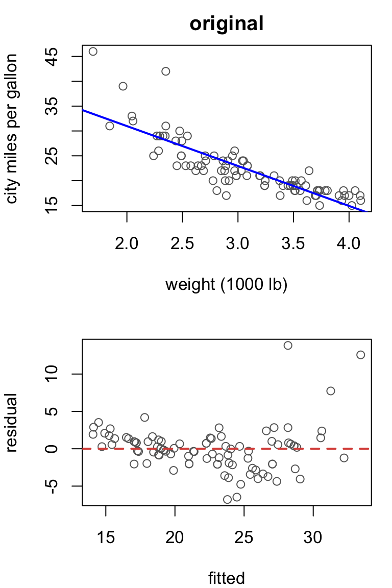
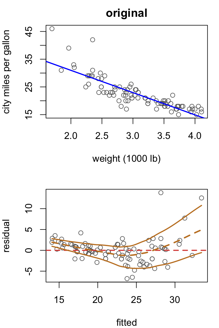
Original model: \[Y_i = \beta_0 + \beta_1 x_i + \epsilon_i\]
Issue: nonlinearity and nonconstant variance.
Transformation: \[\frac{100}{Y_i} = \beta_0 + \beta_1 x_i + \epsilon_i\] Most of the curve and the fan are gone.
Back-transformation
             Estimate Std. Error    t value     Pr(>|t|)
(Intercept) 0.1936667 0.23708840  0.8168544 4.161450e-01
weight      1.4662292 0.07578551 19.3470924 5.265735e-34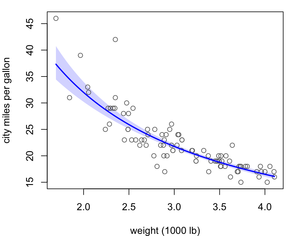
Fitted model: \[\hat{Y}_i = \frac{100}{0.194 + 1.466\, x_i}\]
Here, \(\hat{Y}_i\) estimates the median fuel economy.
On the transformed scale, gallons per 100 miles, each extra 1000 lb adds 1.47.
Each additional 1000 lb is associated with an estimated 1.47 more gallons used per 100 miles, on average.
Box-Cox: trees
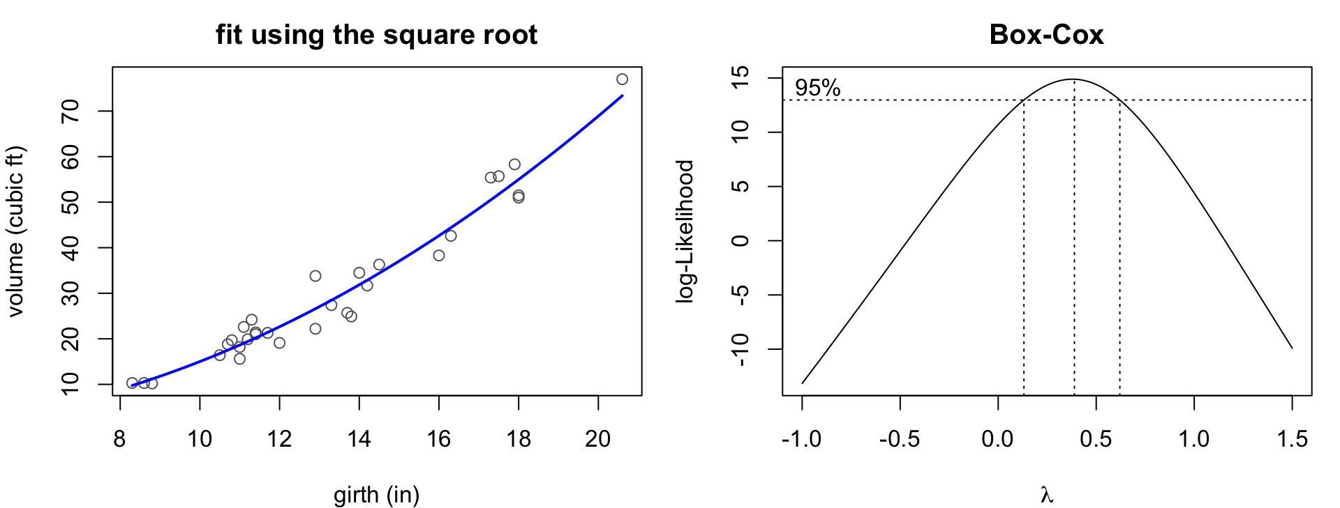
The best power is 0.38, and anything from 0.13 to 0.62 is reasonable. A square root, power \(1/2\), is in that range.
Box-Cox: cars
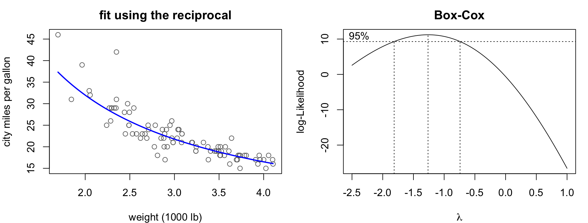
The best power is -1.26, and anything from -1.81 to -0.74 is reasonable. A reciprocal, power \(-1\), is in that range.
Centering and squaring the predictor
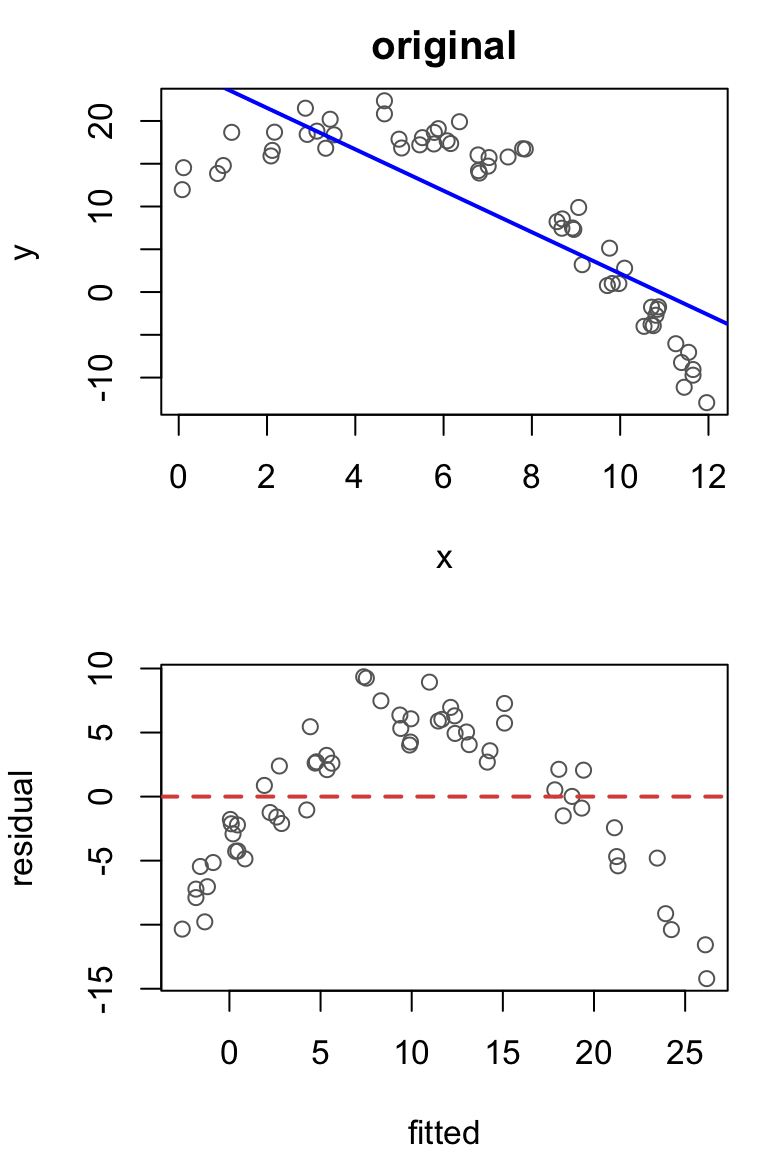
Some relationships rise and then fall, or fall and then rise, and logs and powers can’t straighten those. Here are 60 simulated observations whose trend turns around near \(x = 4\).
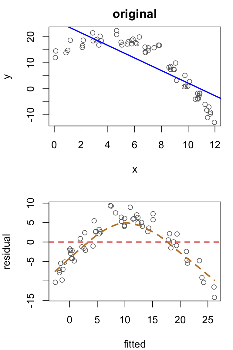
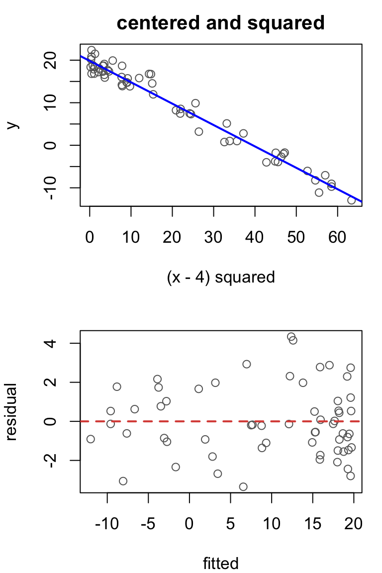
Original model: \[Y_i = \beta_0 + \beta_1 x_i + \epsilon_i\]
Issue: nonlinearity. The trend changes direction.
Transformation: \[Y_i = \beta_0 + \beta_1 (x_i - c)^2 + \epsilon_i\] With \(c = 4\), the curve is gone.
Back-transformation
               Estimate Std. Error   t value     Pr(>|t|)
(Intercept)  19.8322416 0.33641317  58.95204 1.835915e-53
I((x - 4)^2) -0.5027307 0.01175219 -42.77763 1.447942e-45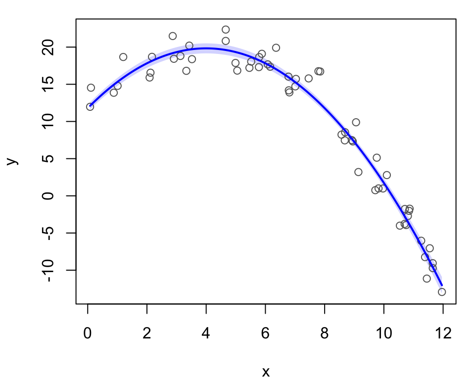
Fitted model: \[\hat{Y}_i = 19.83 -0.503\, (x_i - 4)^2\]
Here, \(\hat{Y}_i\) estimates the mean response.
\(\hat{Y}\) is largest at \(x = 4\) and falls off with the squared distance from 4.
The estimated mean response peaks at 19.83 when \(x = 4\). At a distance \(d\) from 4, it is lower by \(0.503\, d^2\).
Where to center?
The center \(c\) should be where the curve turns.
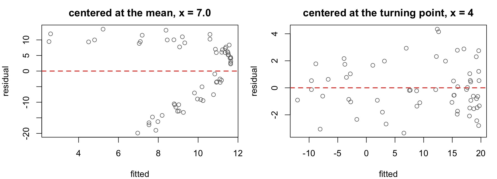
If the turning point is hard to see, don’t guess — you’re adding a model constraint not estimated from the data, so should only do this if the constraint is obvious.
Activity: diagnose and fix
Twelve simulated datasets, each with one predictor. For each one: diagnose the problem, try a fix, and check that the fix worked.
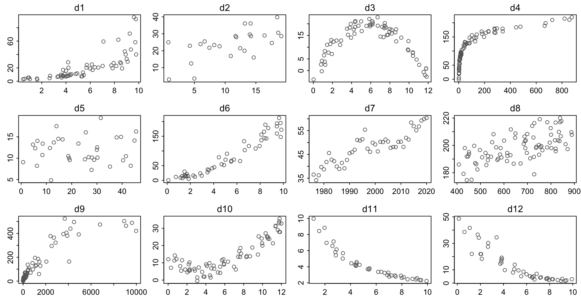
The script is scripts/06-diagnose-and-fix.R on the course site.
Activity: the true models
The solid curve is the trend each dataset was simulated from, and \(\varepsilon\) is the error.
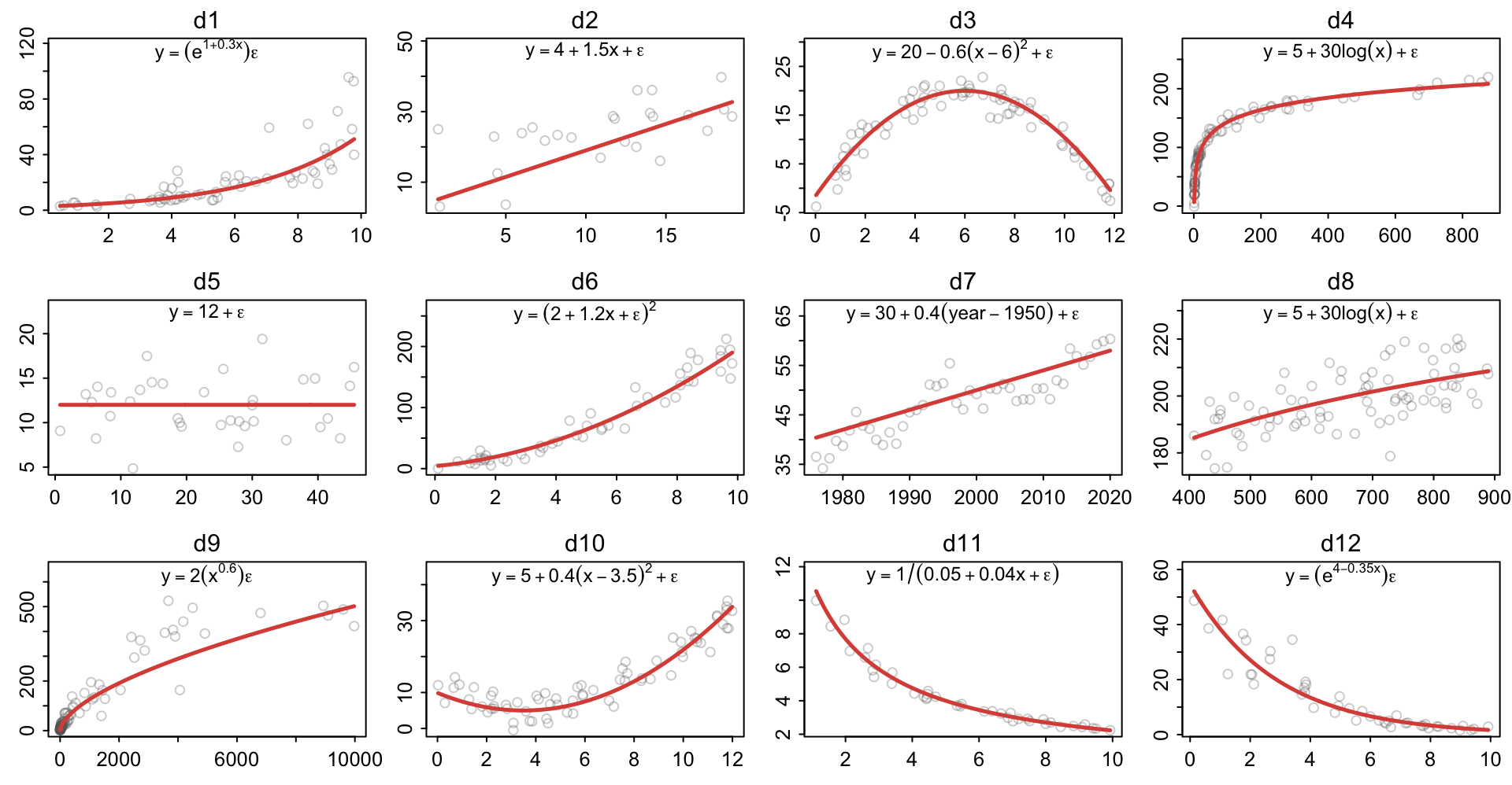
The errors in d7 are correlated: each year’s error carries over into the next.
Unusual observations
Hours of sleep per day against lifespan for 51 species.
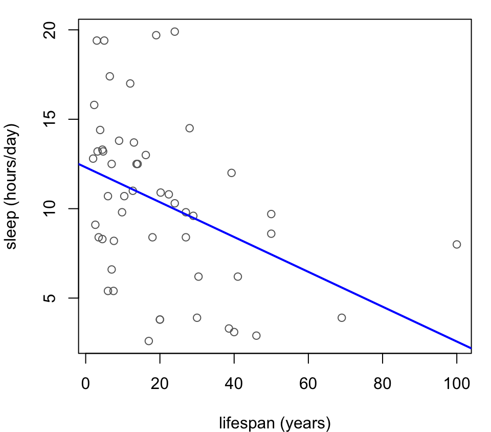
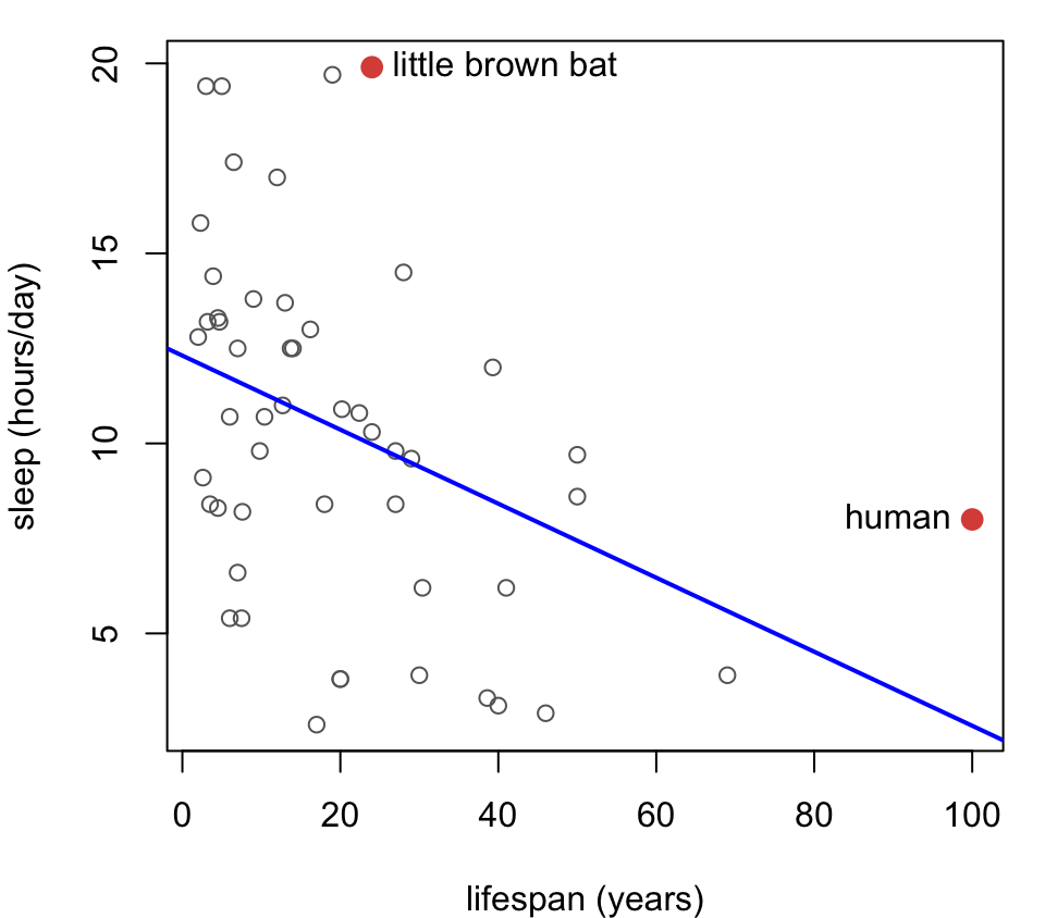
Diagnostics were fine, but a couple of points stood out.
Two points are unusual, and in different ways:
- Humans live far longer than any other species here
- The little brown bat sleeps almost 20 hours a day
Leaving one out
What happens to the fit if we remove each of these points in turn?
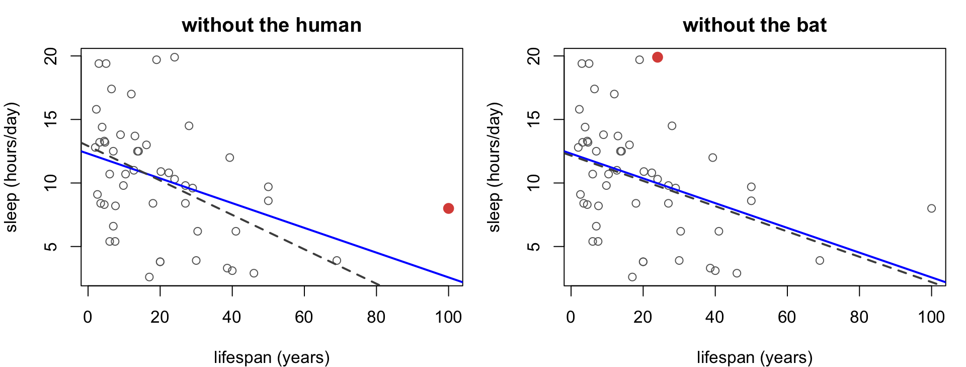
Solid line: all the data. Dashed line: without the red point.
Influence
An influential point is one whose removal noticeably changes the fit.
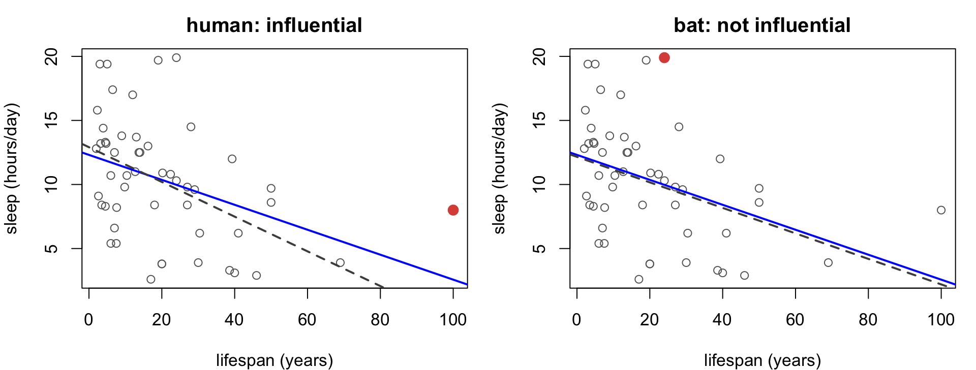
Not all unusual observations are influential:
- removing the human changes the fit a lot
- removing the bat barely changes it
Why the difference? Two factors:
- unusualness in \(x\) or “leverage”
- unusualness in \(Y\) or “outlier”
Leverage
Leverage measures how far an observation’s predictor value is from the center of all the predictor values.
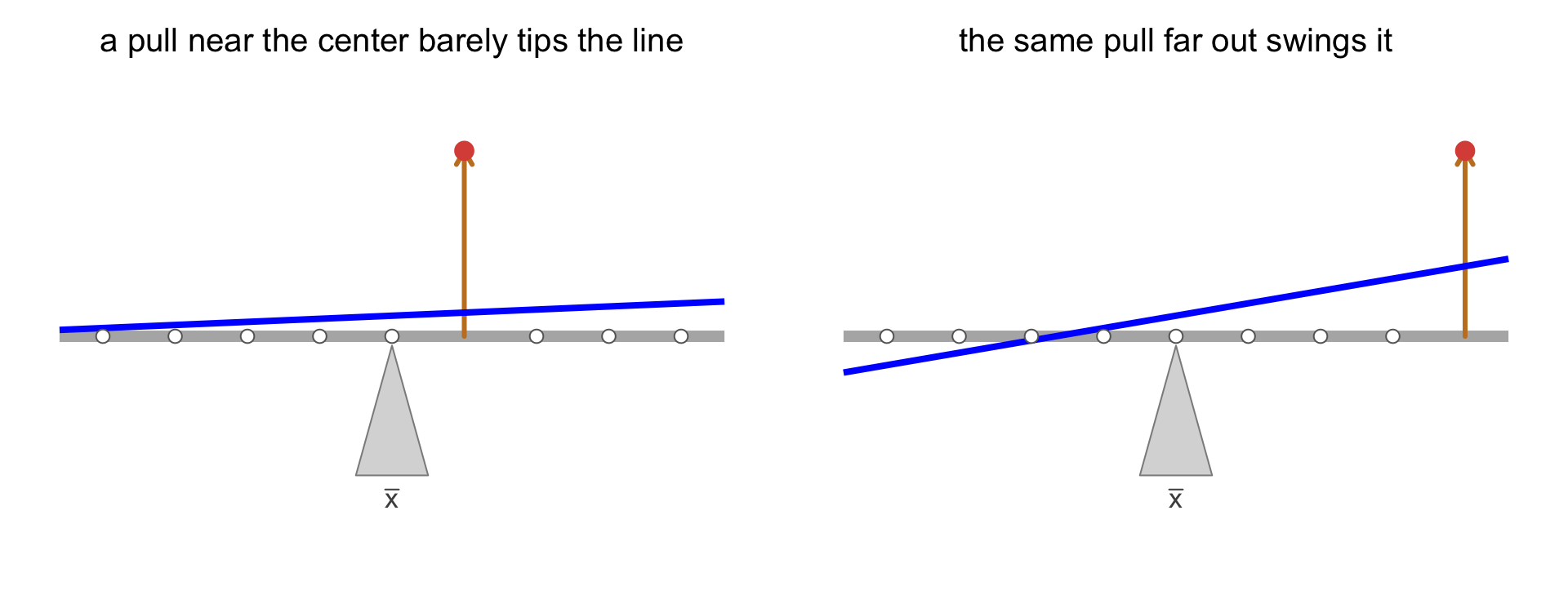
The fit balances on a fulcrum near \(\bar{x}\): the further out an observation sits, the more the line follows it.
Measuring leverage
For simple linear regression, leverage is a squared distance from \(\bar{x}\), measured in standard deviations: \[ h_{ii} = \frac{1}{n} + \frac{1}{n - 1}\left(\frac{x_i - \bar{x}}{s_x}\right)^2 \qquad (i^\text{th} \text{ diagonal of } H) \]
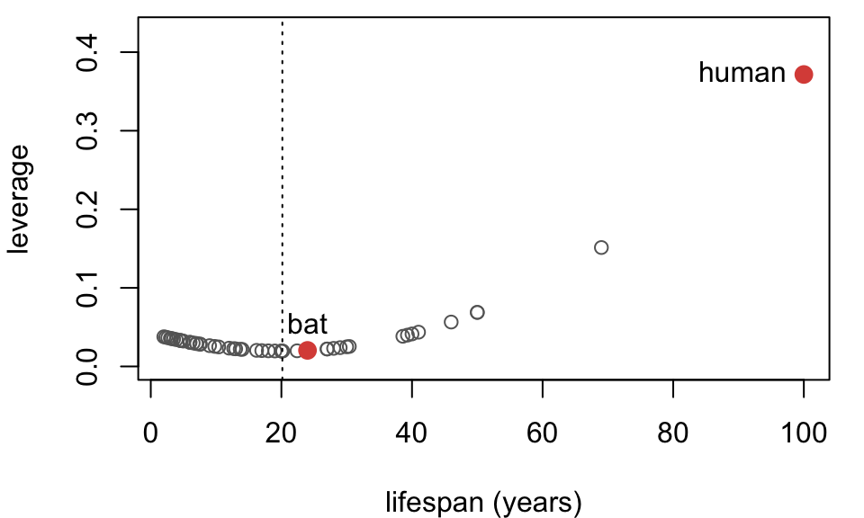
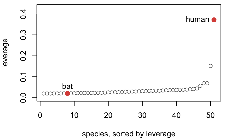
Humans are 4.2 standard deviations above the mean lifespan, so their leverage of 0.372 stands far apart. The bat is close to the mean, with leverage 0.020.
Outliers
An outlier is an observation that doesn’t conform to the model.
In regression:
- outlier = large residual
Consider:
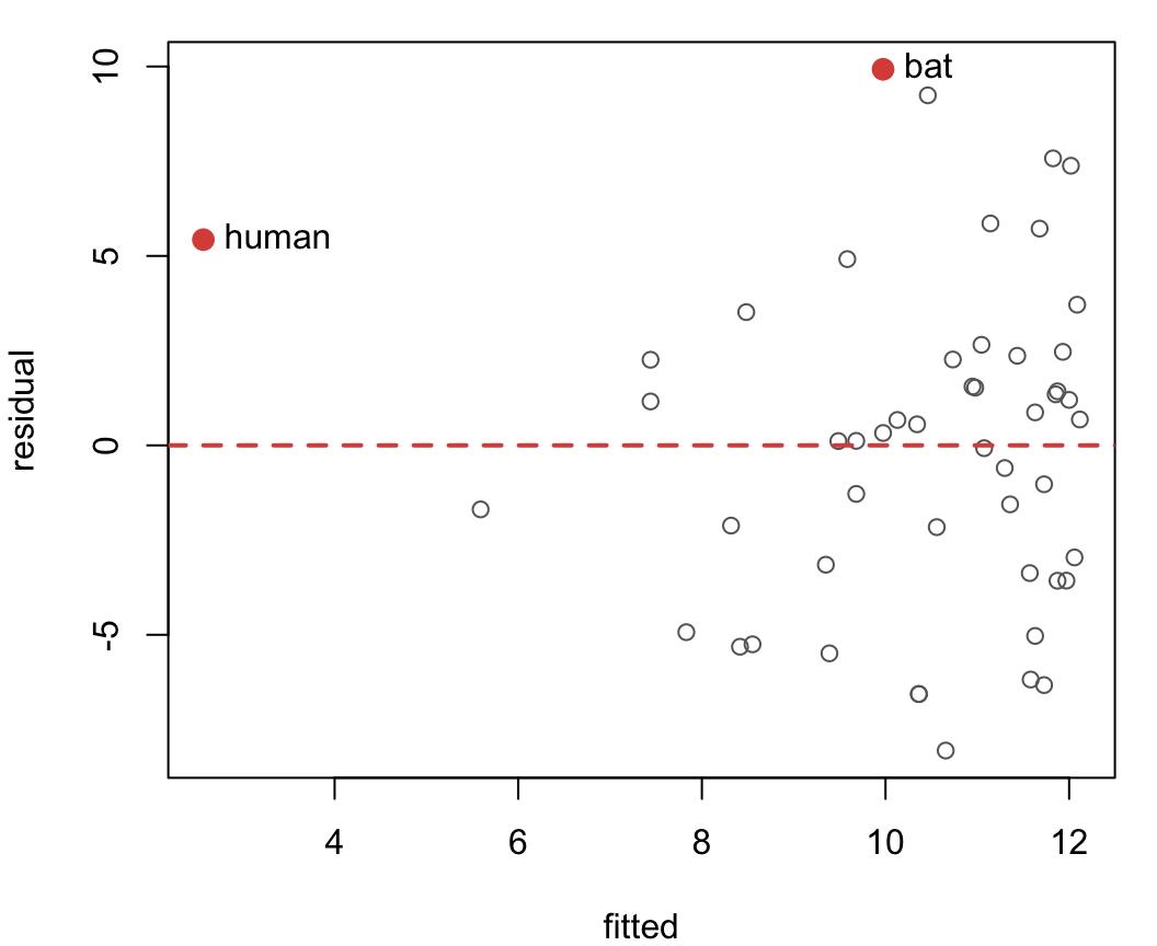
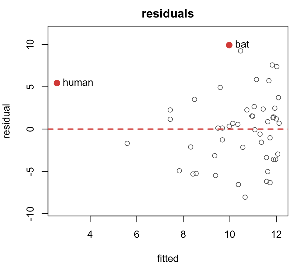
- bat sleeps 9.9h more than predicted
- human sleeps 5.4h more than predicted
But are they outliers? How large is too large?
Studentized residuals
Idea: put the residuals on a standard scale.
Since \(e = (I - H)\epsilon\), residual variance depends on leverage: \[\text{var}[e_i] = \sigma^2 (1 - h_{ii})\]
So we define the studentized residual as: \[r_i = \frac{e_i}{\hat\sigma \sqrt{1 - h_{ii}}}\]
Then look for values in the tails (\(|r_i| > 3\)) and far from the rest.
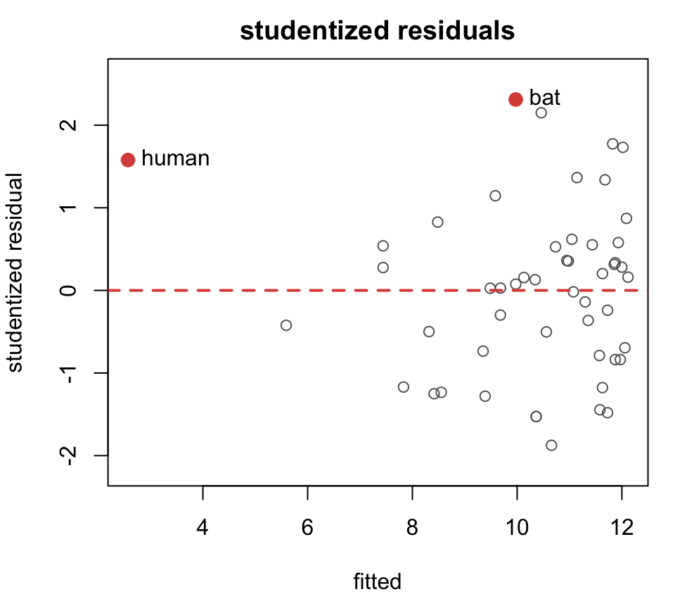
Bat: \(r = 2.31\). Human: \(r = 1.58\). Neither is an outlier.
Measuring influence
Removing observation \(i\) moves its own fitted value by \[\hat{Y}_i - \hat{Y}_{(i)} = h_{ii}\,\big(Y_i - \hat{Y}_{(i)}\big)\] where \(\hat{Y}_{(i)}\) is the fitted value from the fit without observation \(i\).
Cook’s distance measures how much all fitted values move: \[D_i = \frac{\sum_j \big(\hat{Y}_j - \hat{Y}_{j(i)}\big)^2}{2\,\hat\sigma^2}\]
But computing \(n\) separate fits holding out one observation at a time is cumbersome.
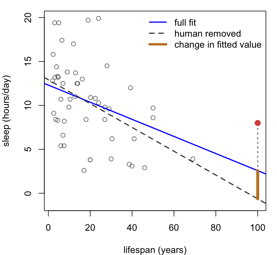
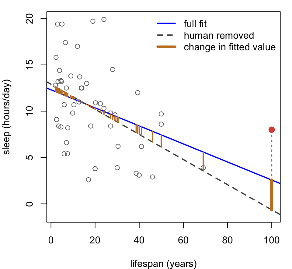
Cook’s distance for the mammals
Little.brown.bat    Water.opossum              Man
0.056 0.056 0.736 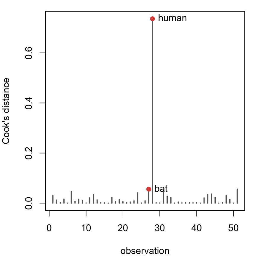
Humans stand far apart from every other species.
But does it matter for inference?
Effect on inference
            Estimate Std. Error t value Pr(>|t|)
(Intercept)  12.3117     0.8896 13.8399    0.000
lifespan -0.0974 0.0322 -3.0212 0.004 Estimate Std. Error t value Pr(>|t|)
(Intercept) 12.9095 0.9517 13.5641 0.0000
lifespan -0.1355 0.0396 -3.4179 0.0013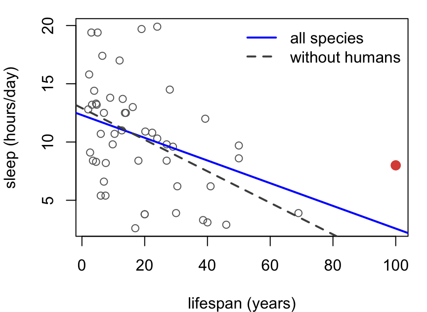
Whether it matters depends on your goal:
- no effect on inferred association
- attenuates slope slightly by half an hour per ten years and within 2SE
- will affect predictions, but only in the right tail at 50+
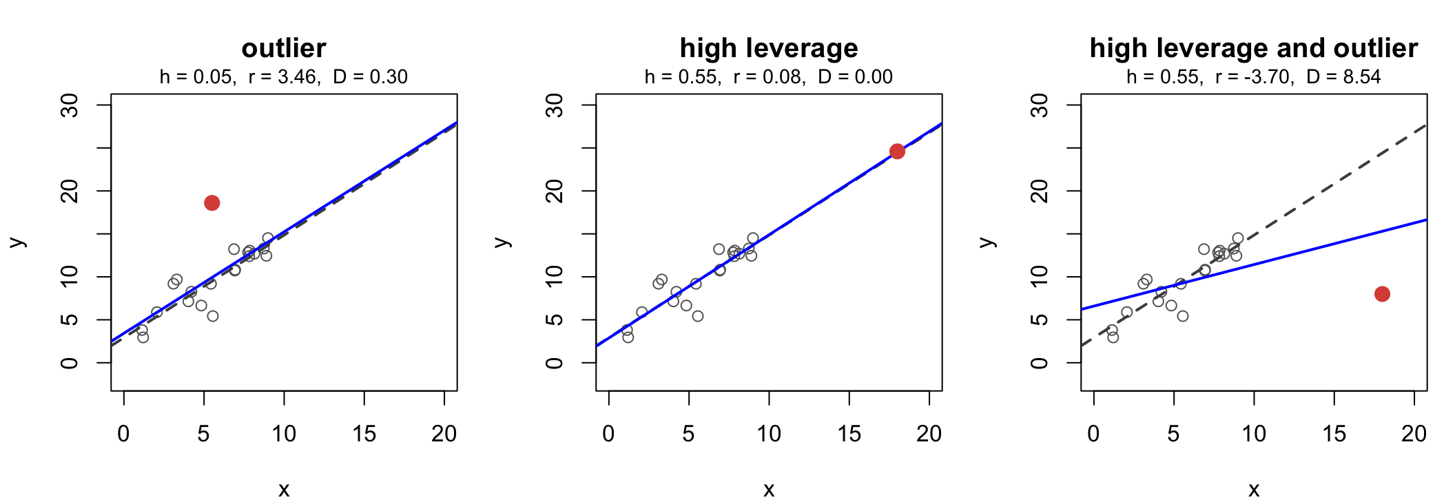
Three kinds of unusual
Solid line: the fit with the red point. Dashed line: the fit without it.
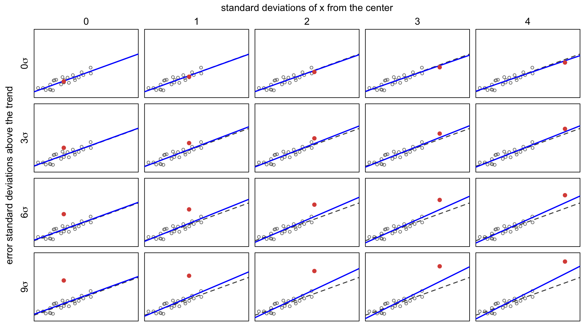
Calibrate your eyes
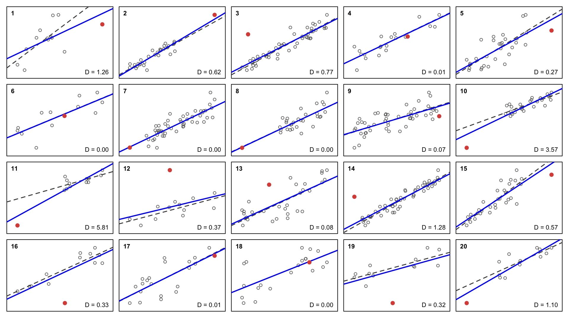
The same 24 points in every panel, plus one red point that moves.
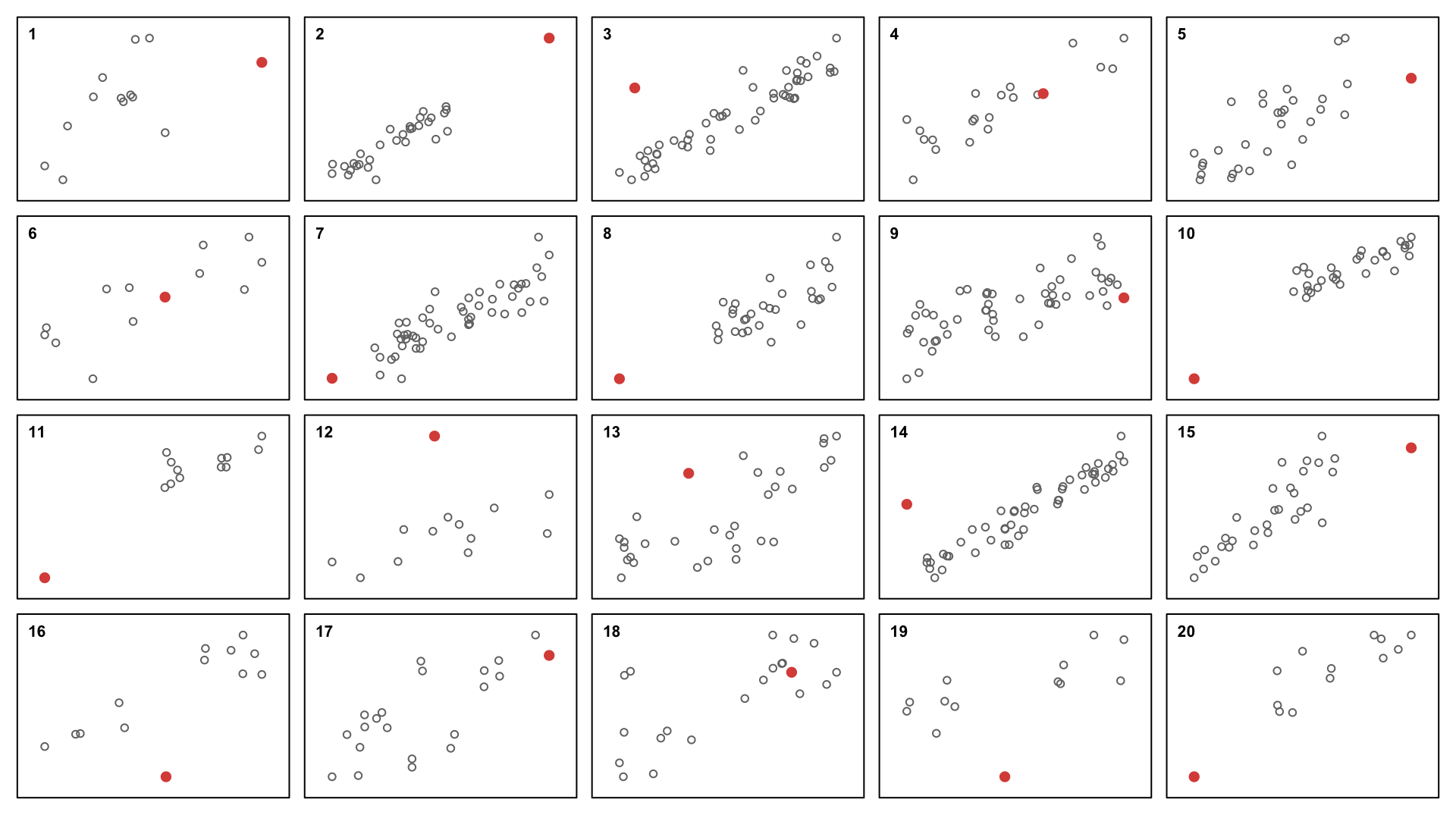
Now try guessing
Which red points are influential? High leverage? High outlyingness?
Check your understanding
Dashed: fit without the red point. Solid: fit with it. Cook’s distance in each corner.