Applied Linear Models

STAT3530 Fall 2026

Review: inference for one mean

Consider \(Y_1, \dots, Y_n \stackrel{iid}{\sim} N(\mu, \sigma^2)\).

The normality entails that

\[ T(\mu) = \frac{\bar Y - \mu}{s_Y/\sqrt{n}} \sim t_{n-1} \]

so we get confidence intervals, e.g.,

• \(\bar Y \pm t^{\alpha/2}_{n-1} \frac{s_Y}{\sqrt{n}}\)

and hypothesis tests of \(H_0: \mu = \mu_0\), e.g.,

• reject when \(|T(\mu_0)| > t^{\alpha/2}_{n-1}\)

Viewed through a regression lens

drag the dot to move the line
μ = —   σ = —   SSE = —
normal curve

Model \(Y = \mu\mathbf{1} + \epsilon\) with \(\epsilon \sim N(0, \sigma^2 I)\).

# estimate mean and se using lm
fit <- lm(body.temp ~ 1, data = temps)
summary(fit)$coefficients[, 1:2]

   Estimate  Std. Error 
98.24923077  0.06430442 

the error normality implies \[ T(\mu) = \frac{\hat\mu - \mu}{SE(\hat\mu)} \sim t_{n-1} \]

so we can do inference, for example

# confidence interval
confint(fit, level = 0.95)

             2.5 %   97.5 %
(Intercept) 98.122 98.37646

The underlying assumption

All of this machinery turns on \(\epsilon\) being normally distributed: \[ \text{error normality} \quad\Longrightarrow\quad \text{response normality} \quad\Longrightarrow\quad \text{estimator normality} \]

or more formally \[ \epsilon \sim N(0, \sigma^2I) \quad\Longrightarrow\quad Y \sim N(\mu, \sigma^2 I) \quad\Longrightarrow\quad \hat{\mu} \sim N\left(\mu, \frac{\sigma^2}{n}\right) \]

For the linear model we have the same pattern \[ \epsilon \sim N(0, \sigma^2I) \quad\Longrightarrow\quad Y \sim N(X\beta, \sigma^2 I) \quad\Longrightarrow\quad \hat{\beta} \sim N\left(\beta, \sigma^2 (X^TX)^{-1}\right) \] only with slightly longer expressions.

Inference in regression

Now for \(Y = X\beta + \epsilon\) with \(\epsilon \sim N(0, \sigma^2 I)\)

fit <- lm(force ~ height, data = crab)
summary(fit)$coefficients[, 1:2]

              Estimate Std. Error
(Intercept) -11.086902   4.622402
height        2.634823   0.508917

the error normality implies \[ T_j = \frac{\hat\beta_j - \beta_j}{SE(\hat\beta_j)} \sim t_{n-2} \]

so we can do inference, for example

confint(fit)

                 2.5 %    97.5 %
(Intercept) -20.461568 -1.712237
height        1.602692  3.666955

drag the dots to move the line
β₀ = —   β₁ = —   σ = —   SSE = —
normal curves

Significance tests

Is the predictor doing anything at all? \[ H_0: \beta_1 = 0 \quad\text{vs}\quad H_a: \beta_1 \neq 0 \]

Under \(H_0\) and error normality we have \[ T_1 = \frac{\hat\beta_1 - 0}{SE(\hat\beta_1)} \sim t_{n-2} \]

so we reject when \(|T_1| > t^{\alpha/2}_{n-2}\) or

\[\underbrace{2P\left(t_{n-2} > |T_j|\right)}_\text{p-value} < \alpha\]

# check second row
summary(fit)$coefficients

              Estimate Std. Error   t value     Pr(>|t|)
(Intercept) -11.086902   4.622402 -2.398515 2.176729e-02
height        2.634823   0.508917  5.177314 8.730239e-06

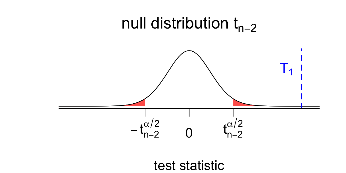
Interpretation: the data suggest that mean closing force is associated with claw height.

Confidence intervals

A \((1 - \alpha)\times 100\%\) confidence interval is \[ \hat\beta_1 \pm t^{\alpha/2}_{n-2}\,SE(\hat\beta_1) \]

Could do manually:

# estimates for crab data
summary(fit)$coefficients[, 1:2]

              Estimate Std. Error
(Intercept) -11.086902   4.622402
height        2.634823   0.508917

critical value \(t^{0.025}_{36} = 2.028\) gives \[ 2.635 \;\pm\; 2.028 \times 0.509 = (1.6, 3.7) \]

Or in R:

# intervals for coefficients
confint(fit, level = 0.95)

                 2.5 %    97.5 %
(Intercept) -20.461568 -1.712237
height        1.602692  3.666955

Interpretation. With 95% confidence, each additional mm of claw height is associated with an increase in mean closing force of between 1.6 and 3.7 newtons.

Example

Recall the RFFT data.

# fit the model and check estimates
fit <- lm(rfft ~ age, data = prevend)
summary(fit)$coefficients

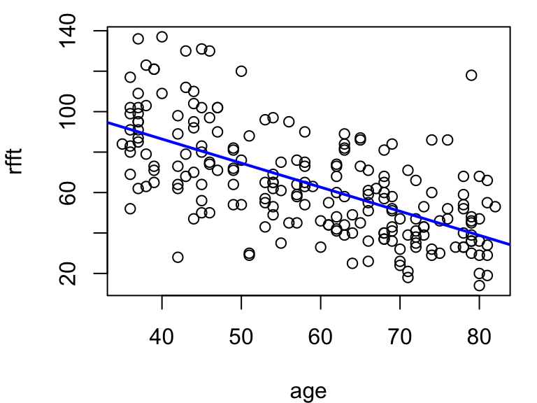
              Estimate Std. Error   t value     Pr(>|t|)
(Intercept) 134.098052  6.0700593  22.09172 3.058596e-56
age          -1.190794  0.1007061 -11.82445 5.823319e-25

# confidence intervals
round(confint(fit), 3)

              2.5 %  97.5 %
(Intercept) 122.131 146.065
age          -1.389  -0.992

Your turn:

1. Is cognitive function significantly associated with age?
2. Interpret the confidence interval.

New values

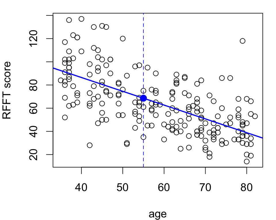
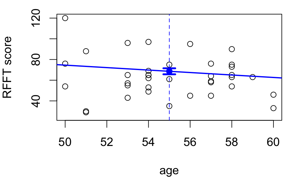
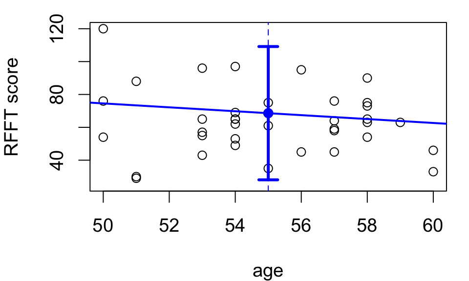
Consider the plug-in estimate \(x_0^T \hat\beta\) at a new value \(x_0\). For example:

# model estimate for a 55 year old
predict(fit, newdata = data.frame(age = 55))

       1 
68.60439 

This computes: \[ 134.098 - 1.1908 \times 55 = 68.604 \]

There are two possible estimands here:

1. a new observation \(Y_0 = x_0^T \beta + \epsilon\)
2. the average response \(\mu_0 = \mathbb{E}[Y_0] = x_0^T\beta\)

Possible estimands

The point estimate is the same: \(\hat{Y}_0 = x_0^T\hat\beta\). Consider its variance: \[ \text{var}\left[\hat{Y}_0\right] = \text{var}\left[x_0^T\hat\beta\right] = x_0^T \text{var}\left[\hat\beta\right] x_0 = x_0^T \left[\sigma^2 (X^TX)^{-1}\right] x_0 = \sigma^2 \underbrace{x_0^T (X^TX)^{-1} x_0}_{h_{00}} \]

Now consider the variance relative to each estimand:

as an estimate of \(\mu_0\) we have \[ \text{var}\left[\hat{Y}_0 - \mu_0\right] = \text{var}\left[\hat{Y}_0\right] = \sigma^2 h_{00} \]

giving standard error \[ SE(\hat{Y}_0) = \hat\sigma^2 h_{00} \]

but as an estimate of \(Y_0\) we have \[ \text{var}\left[\hat{Y}_0 - Y_0\right] = \text{var}[\hat{Y}_0] + \text{var}\left[Y_0\right] = \sigma^2 h_{00} + \sigma^2 \]

giving standard error \[ SE(\hat{Y}_0) = \hat\sigma^2 (1 + h_{00}) \]

Confidence interval for the mean

Thus, two interpretations:

1. The estimated mean RFFT score for 55 year olds is 68.6
2. The predicted value of RFFT for a specific 55 year old is 68.6

predict(fit, newdata = data.frame(age = 55),
        interval = 'confidence',
        level = 0.95)

       fit     lwr      upr
1 68.60439 65.7101 71.49868

Prediction interval

Two readings of the same prediction:

1. The estimated mean RFFT score for 55 year olds is 68.6
2. The predicted value of RFFT for a specific 55 year old is 68.6

predict(fit, newdata = data.frame(age = 55),
        interval = 'prediction',
        level = 0.95)

       fit      lwr      upr
1 68.60439 28.04903 109.1598

Uncertainty bands

Computing an interval at every \(x\) gives a band.

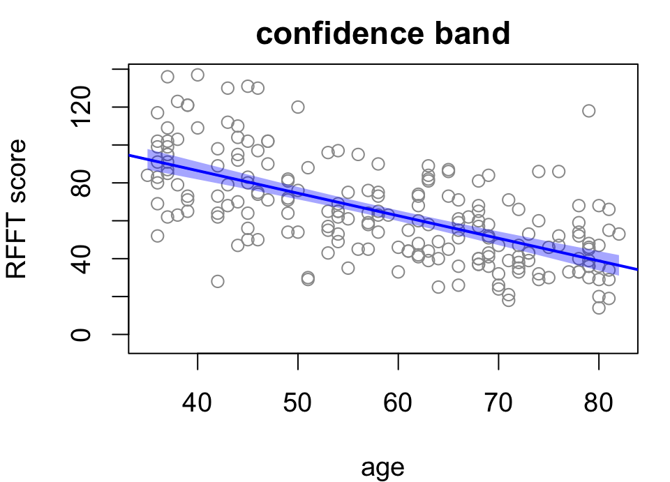
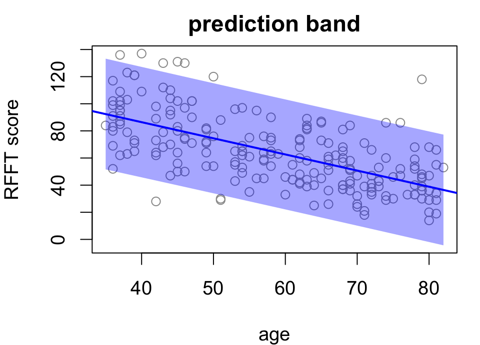
Individual observations are more variable than averages.

Which is which?

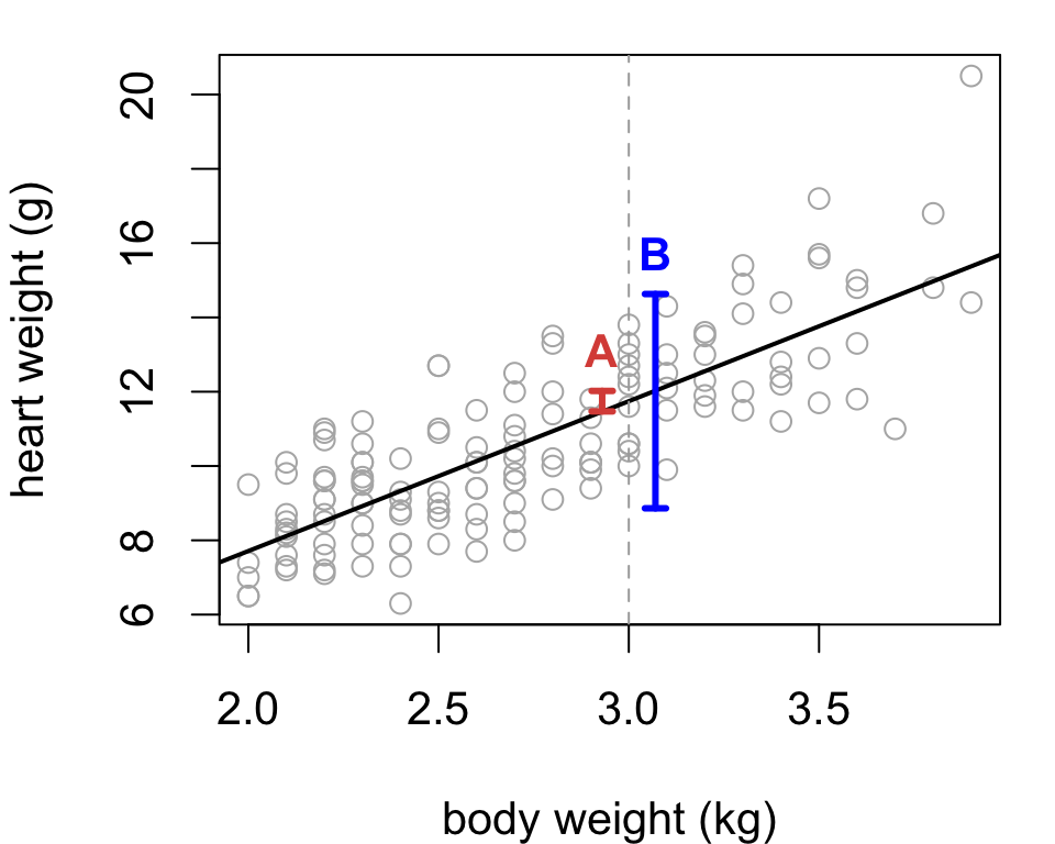
The cats data from HW2.

Your turn:

1. One interval is for the mean heart weight of 3 kg cats, the other for the heart weight of one 3 kg cat. Which is which?

2. The intervals are \[(11.47,\; 12.02) \quad\text{and}\quad (8.86,\; 14.63)\] Write a sentence interpreting each.

3. Which one would you use to decide whether a 3 kg cat with a 17 g heart is unusual?

Model assumptions

The foregoing depends on four model assumptions.

1. Linearity. The mean response is a linear function of the parameters: \(\mathbb{E}[Y] = X\beta\).

2. Independence. Model errors are independent: \(\epsilon_i \perp \epsilon_j\).

3. Constant variance. The error variance is the same regardless of \(x\): \(\text{var}[\epsilon_i] = \sigma^2\).

4. Normality. Errors are normally distributed: \(\epsilon_i \sim N(0, \sigma^2)\).

Note these are all about the errors. (Linearity is equivalent to \(\mathbb{E}[\epsilon] = 0\).)

Now \(\epsilon\) is unknown, but since \(e = (I - H)\epsilon\) is an observable projection, we perform residual diagnostic checks to look for failures of model assumptions.

Residuals vs fitted values

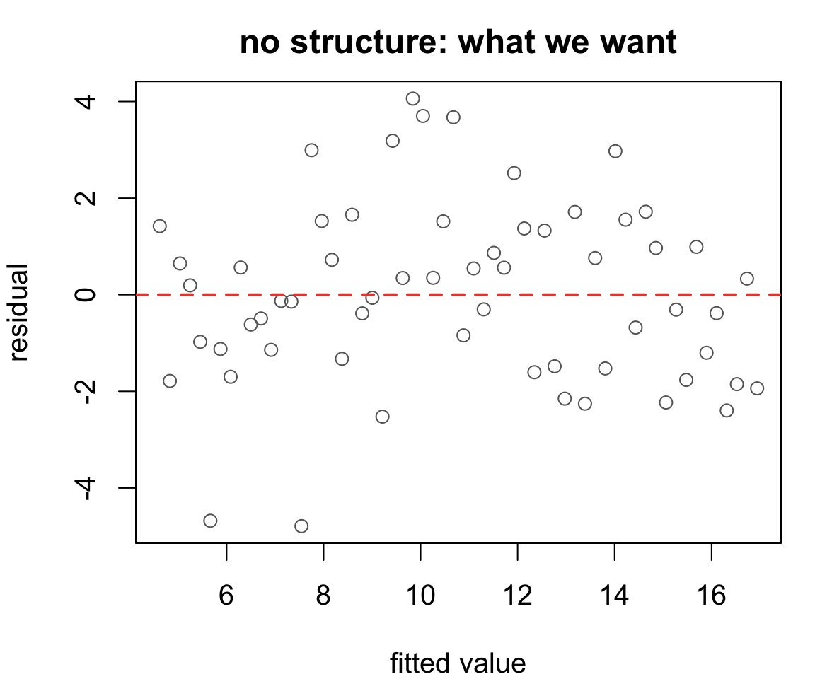
The workhorse plot. Anything you can describe in words is a problem.

In particular, look for:

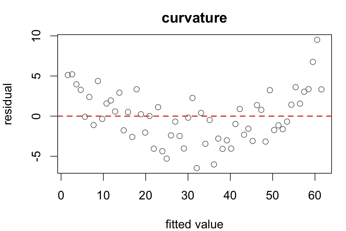
• linearity \(\Rightarrow\) no trend or curve
• constant variance \(\Rightarrow\) even vertical spread
• independence \(\Rightarrow\) no “runs”

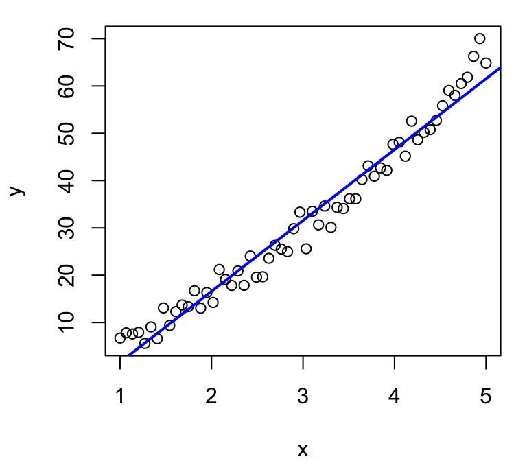
Nonlinearity

Data generated from a quadratic relationship.

Diagnostic shows bowed residuals: positive at the ends, negative in the middle.

Nonconstant variance

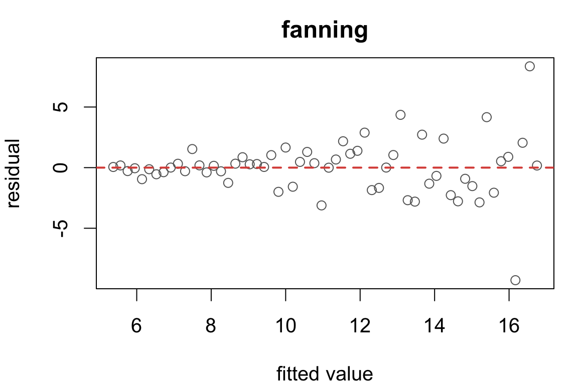
Data generated with variance growing in \(x\).

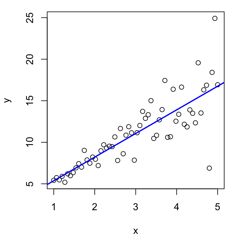
Diagnostic shows a fan or funnel pattern.

Non-normality

Sort the residuals and plot them against normal quantiles in a QQ plot. Normal residuals fall on the \(y = x\) line; read the ends, not the middle.

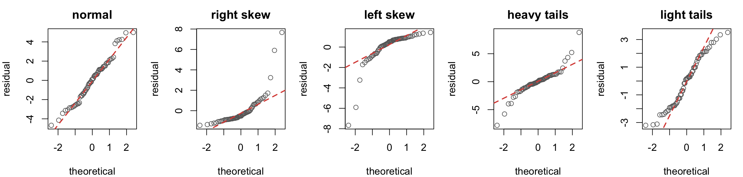
• right skew — both ends bend up
• left skew — both ends bend down

• heavy tails — ends pull away
• light tails — ends flatten

Correlated residuals

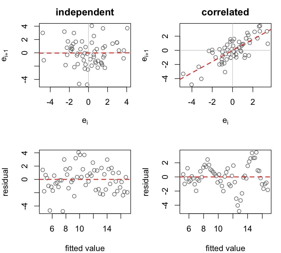
Assumption 2 is the hardest to see, because it is about pairs. No standard diagnostic.

Plotting adjacent residuals can sometimes help spot serial correlation, which also appears as “runs” in the residual versus fit plot.

But there are many other ways that independence can fail.

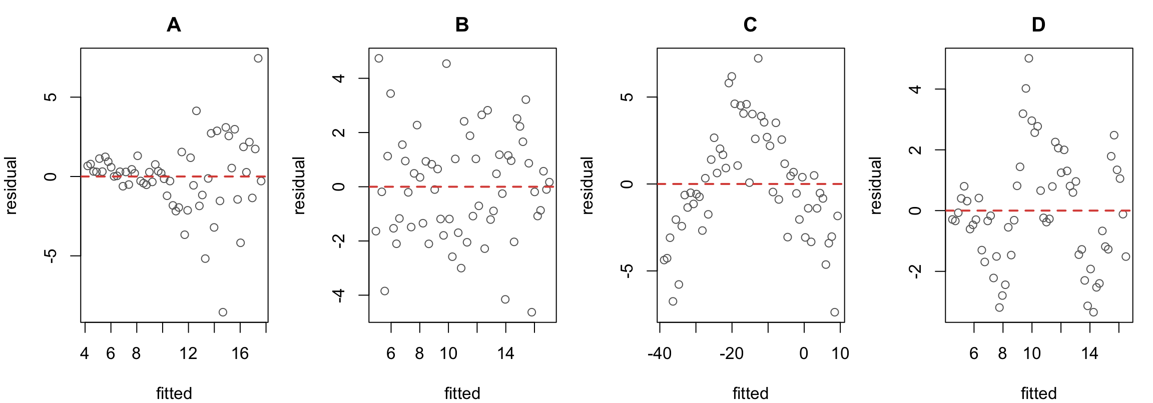
Spot the issue

Each panel is a residual plot from a different fit.

Do the assumptions hold? If not, which one fails?

Spot the issue

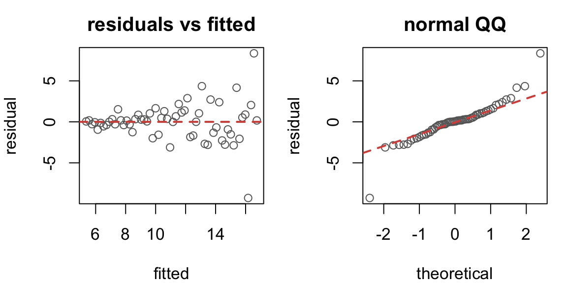
1. Which assumption is violated, and which plot shows it?

2. Is \(\hat\beta_1\) still unbiased here?

3. Is its reported standard error still right?

Consequences

Three of the four failures leave \(\hat\beta\) unbiased.

Only nonlinearity breaks that, and so is arguably the most important assumption.

Assuming linearity holds, the main consequences of other failures are:

• nonconstant variance \(\Rightarrow\) standard errors are wrong
• correlation \(\Rightarrow\) standard errors are wrong
• nonnormality \(\Rightarrow\) confidence intervals and p-values are inexact

All of these affect inference, but in different ways and to different degrees.

Consequences, measured

Each row shows results of simulating 2000 datasets and constructing a CI for \(\beta_1\).

	CI coverage	true SD	reported SE	ratio
well behaved	94.30	0.220	0.220	0.998
heavy tails	95.65	0.220	0.208	0.946
light tails	94.45	0.220	0.220	0.998
variance, mild	94.45	0.248	0.234	0.943
variance, pronounced	87.80	0.562	0.428	0.762
correlation, mild	80.65	0.328	0.214	0.654
correlation, pronounced	46.95	0.584	0.190	0.326

More data helps none of these. It shrinks the interval at the wrong rate.

Assumption hierarchy

Inference is fairly robust to minor issues with model assumptions.

So diagnostic checks should only be sensitive to major failures.

Then, in order of approximate importance:

1. Linearity
2. Correlation
3. Nonconstant variance
4. Normality

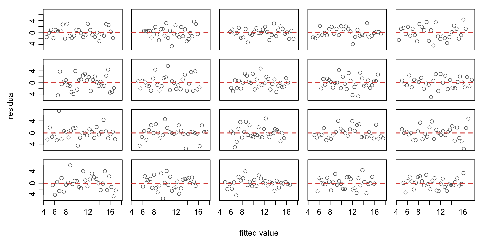
Calibrate your eyes: residuals vs. fit

Twenty fits that satisfy every assumption exactly.

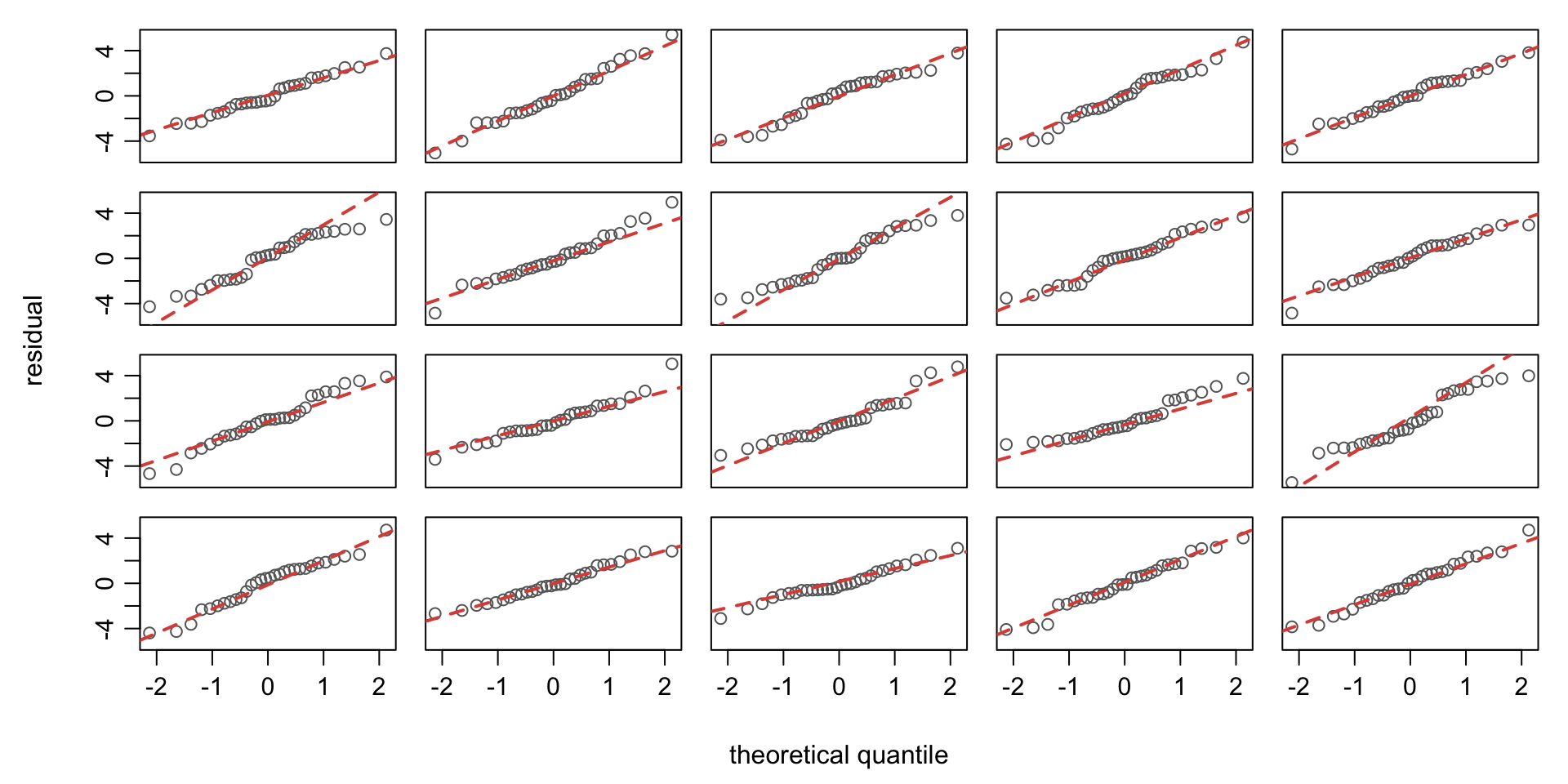
Calibrate your eyes: QQ plots

Another twenty fits that satisfy assumptions exactly.

Examples: mammal sleep

Hours of sleep per day against lifespan, for 51 species.

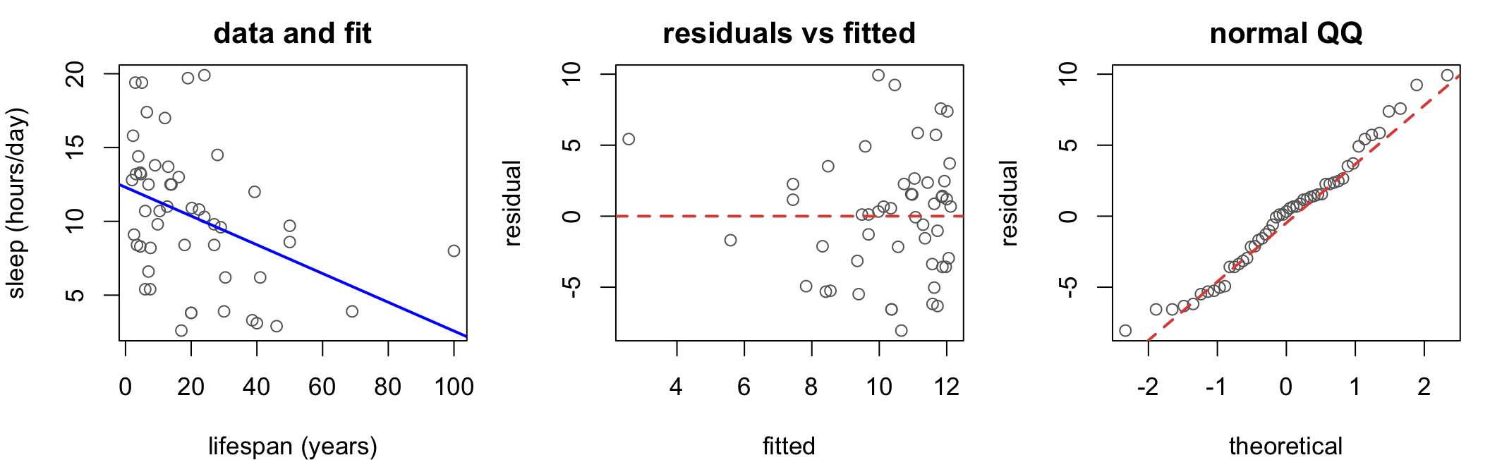
Nothing to report. The model is uninformative but looks correctly specified.

Examples: ozone and temperature

Daily ozone against temperature in the Los Angeles basin, 330 days.

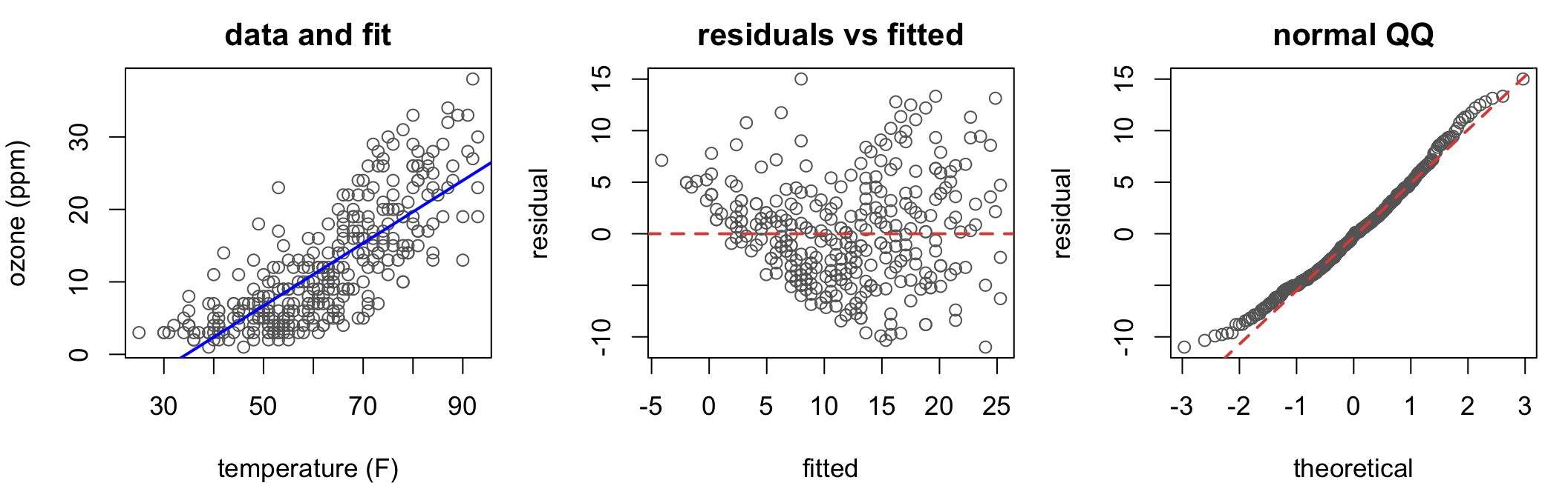
Hard to judge because of the light left tail, which appears because ozone is nonnegative.

But everything is questionable here. Curvature + fanning + light tail.

Also, daily data might be serially correlated.

Examples: ozone and temperature

We should fix other problems first, but might as well check the correlation.

The rows are consecutive days, so plot the residuals in that order.

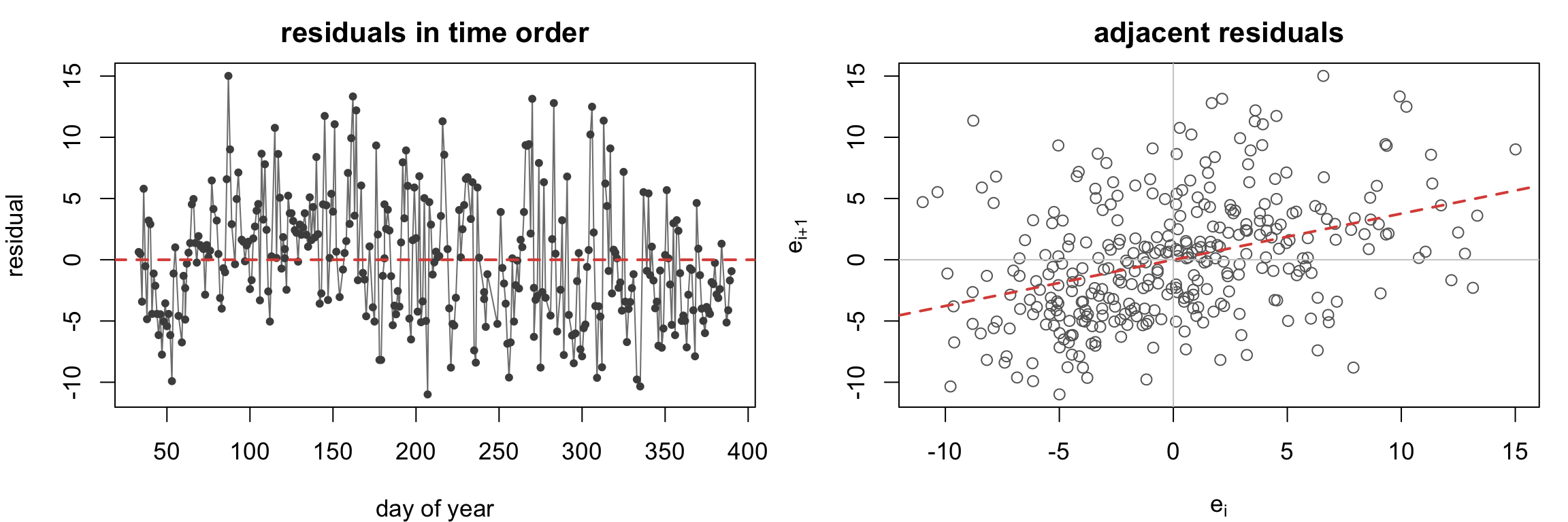
Weakly correlated at 0.38 over one time lag. Independence fails here too.

Example: black cherry trees

Timber volume against trunk girth for 31 felled black cherry trees.

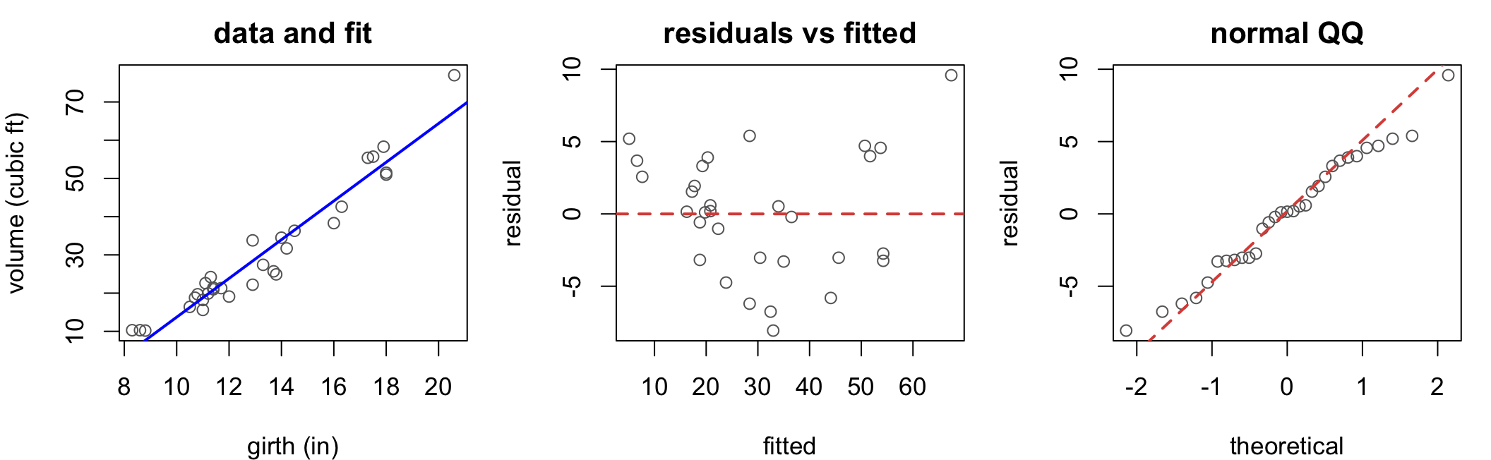
Linearity is questionable here. But since \(\text{vol}\propto \text{girth}^2\), I’d probably revise the model.

Example: endemic species

Proportion of each Galapagos island’s species that are endemic, against log area.

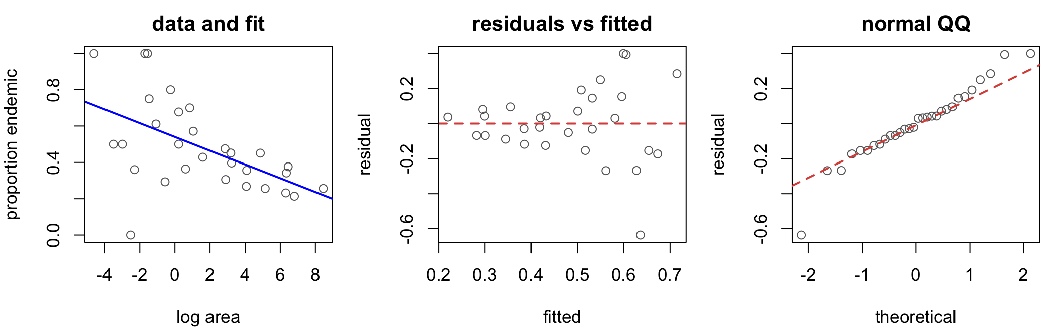
Constant variance fails here: very clear fan pattern.

Example: Lake Huron

Annual level of Lake Huron, 1875–1972, regressed on year.

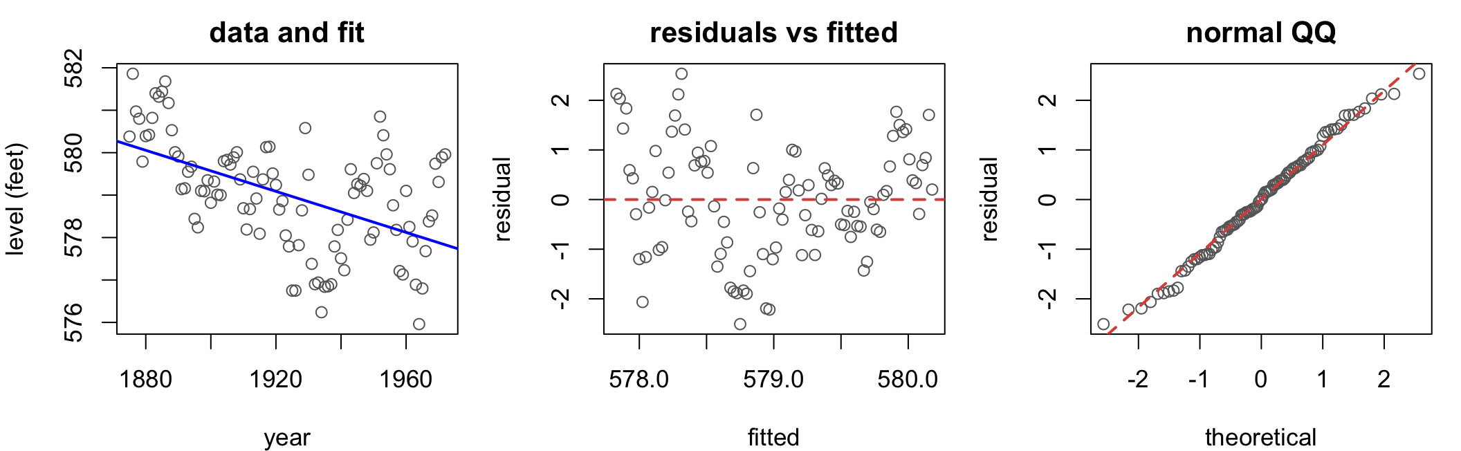
Nothing to report here. But adjacent years might be correlated…

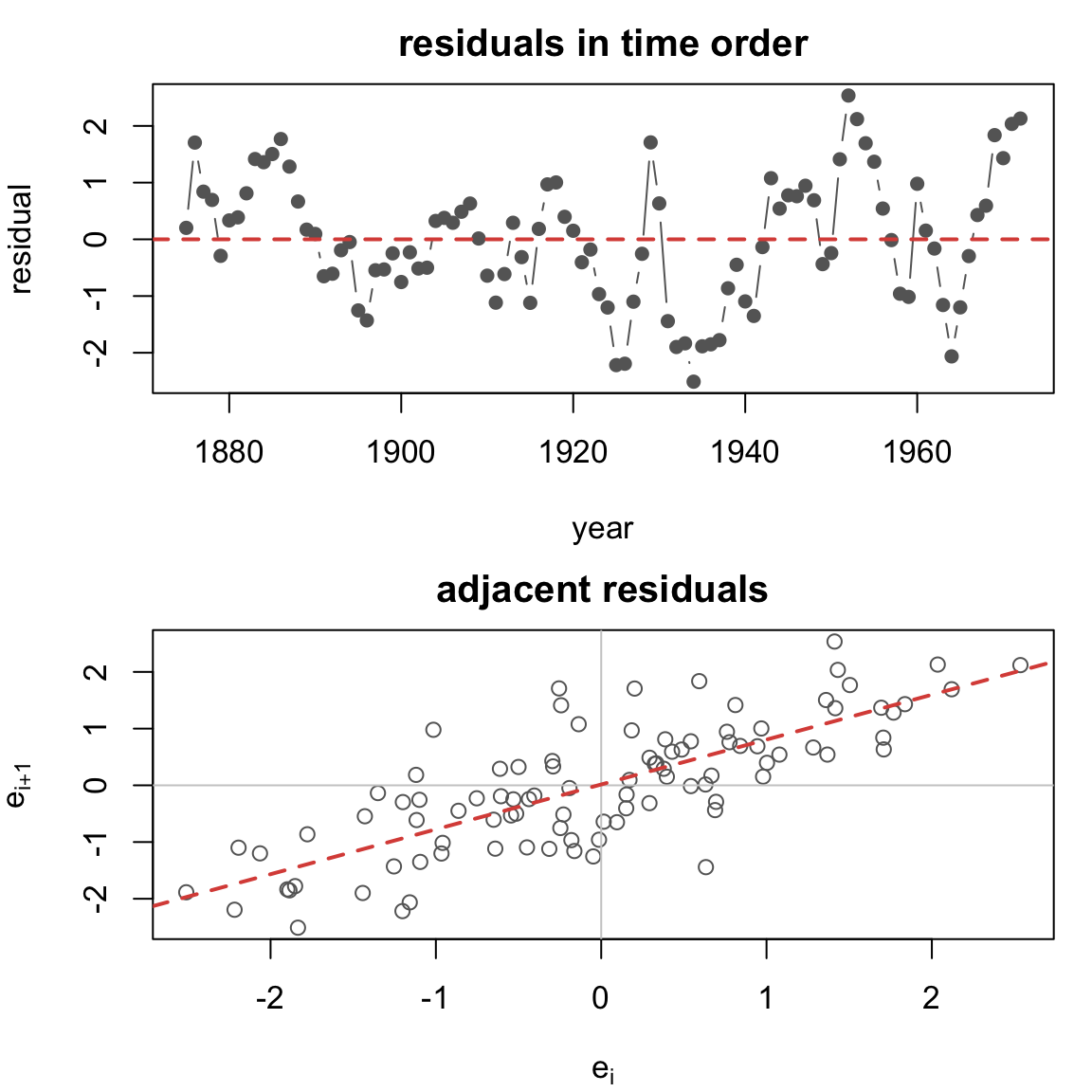
Example: Lake Huron

Correlation is invisible in the standard plot because it is a statement about pairs.

Order the residuals and it appears at once.

Serial correlation is common with time series data — assume it’s present unless you can show otherwise.

Troubleshooting

Once you identify an issue, what to do? Three options:

1. If minor, note it and move on.
2. Transform the data.
3. Model the departure explicitly.

Transformations

The basic idea: find a suitable transformation and fit the model on the transformed scale.

Usually used to fix either nonlinearity or nonconstant variance.

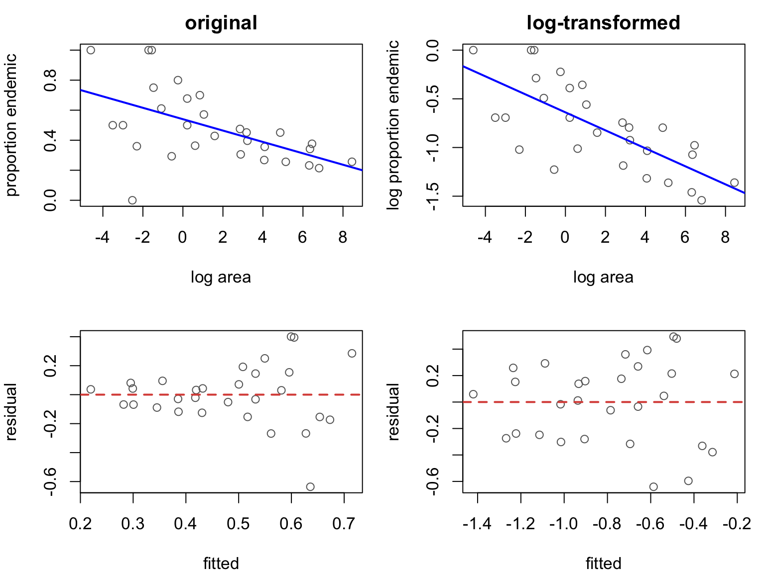
Original model: \[ Y_i = \beta_0 + \beta_1 x_i + \epsilon_i \] After log-transforming the response: \[ \log(Y_i) = \beta_0 + \beta_1 x_i + \epsilon_i \] Residual variance looks much better.

Transformations change the model

If we “undo” the log-transformation \[ \log(Y_i) = \beta_0 + \beta_1 x_i + \epsilon_i \quad\Longleftrightarrow\quad Y_i = e^{\beta_0}\times e^{\beta_1 x_i} \times e^\epsilon_i \] we see the consequences:

• mean response scales exponentially in the predictor
• errors are multiplicative on the original scale
• parameter interpretations change
• assumptions are less transparent

Back-transformation

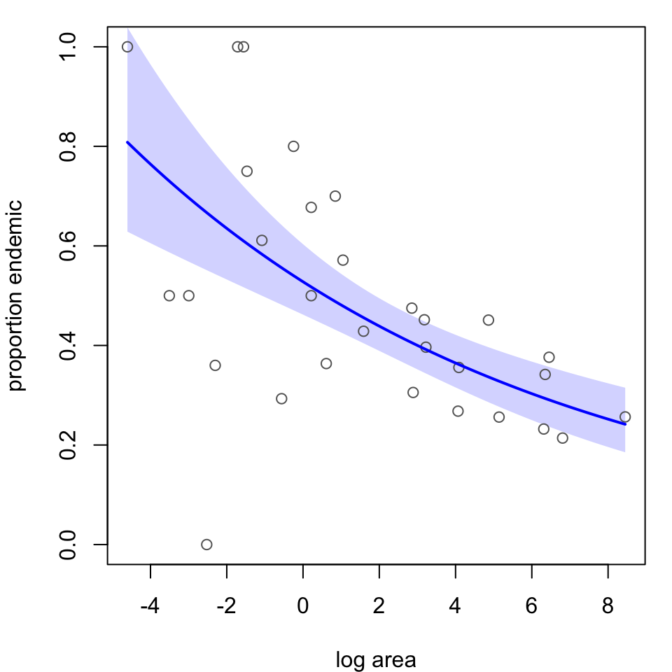
Let’s back-transform the model of the Galapagos data.

# fit on transformed scale
fit <- lm(log(prop) ~ la, 
          data = endemics, 
          subset = keep)
summary(fit)$coefficients

               Estimate Std. Error   t value     Pr(>|t|)
(Intercept) -0.63875781 0.06513603 -9.806521 2.155528e-10
la          -0.09246658 0.01708572 -5.411920 1.009005e-05

So the fitted model is \[ \hat{Y}_i = \underbrace{0.528}_{e^{-0.6388}}\, e^{-0.0925\, x_i} \]

But…

• how should we interpret inferences?
• what do the model assumptions mean?

Interpretation after log transform

Fact: if \(\log(Y) \sim N(\mu, \sigma^2)\) then \(Y\) is lognormal and \(e^\mu\) is the median (not the mean).

So…

• \(\mathbb{E}\left[\log(Y_i)\right] = \beta_0 + \beta_1 x_i \;\Longrightarrow\; \text{median}(Y_i) = e^{\beta_0}e^{\beta_1x_i}\)
• \(e^{\beta_0}\) is the median when \(x_i = 0\)
• \(x_i \to x_i + 1\) changes the median by a factor of \(e^{\beta_1}\)

And inference is for multiplicative change in median per unit change in predictor.

Interpretation after log transform

# fit and back-transform CIs
fit <- lm(log(prop) ~ la, 
          data = endemics, 
          subset = keep)
confint(fit) |> exp()

                2.5 %    97.5 %
(Intercept) 0.4619004 0.6034394
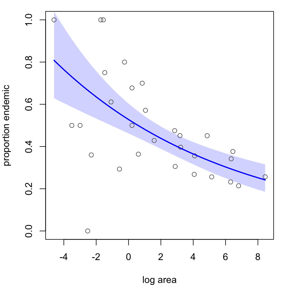
la          0.8802727 0.9442073

• median share of endemic species on a 1km\(^2\) island is estimated to be between 46.2% and 60.3%
• for each one-unit increase in log area, the median share of endemic species is estimated to decrease by between 5.6% and 11.2%

But wait… \(x_i\) here is log area, so there’s another transformation!

Log-transforming the predictor

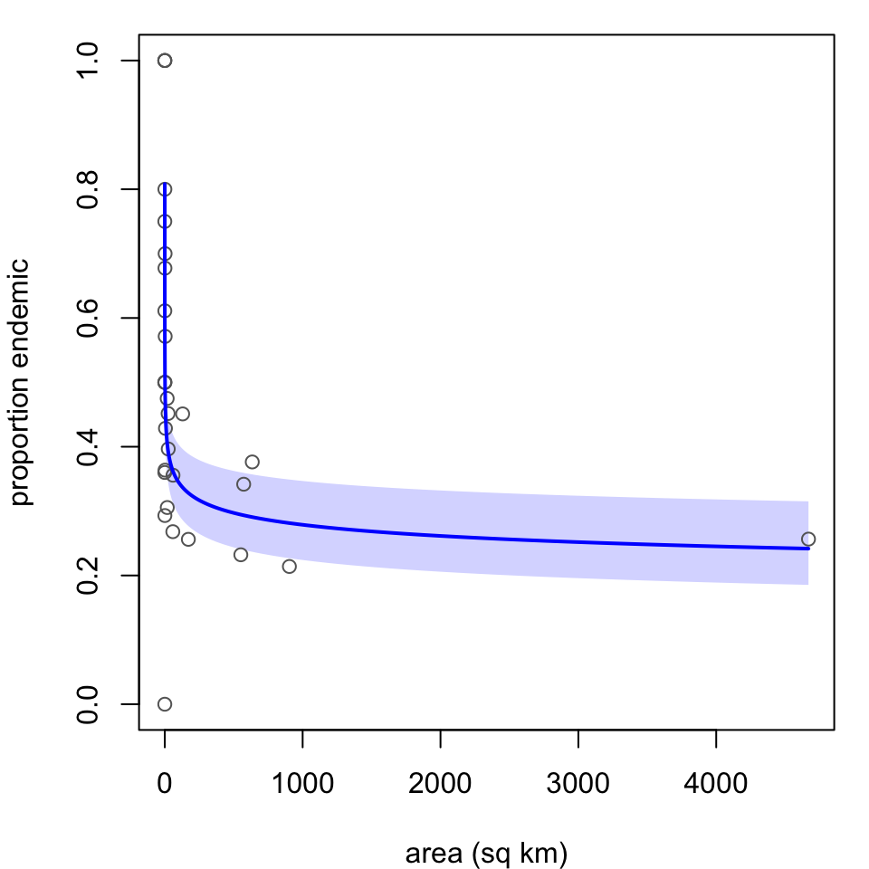
So actually the model is a power law \[ Y_i = e^{\beta_0} \times x_i^{\beta_1} \times e^{\epsilon_i} \] and \(x_i \to 2\, x_i\) means \(Y_i \to 2^{\beta_1}\, Y_i\).

# transform CI
rev(1 - 2^confint(fit)[2, ])

    97.5 %      2.5 % 
0.03901193 0.08459859 

With 95% confidence, every doubling of island area is associated with an estimated 3.9-8.5% decrease in the median share of endemic species.

Diagnostics after transformation

Remember, the model assumptions remain on the transformed scale.

So that is where diagnostics should be assessed.

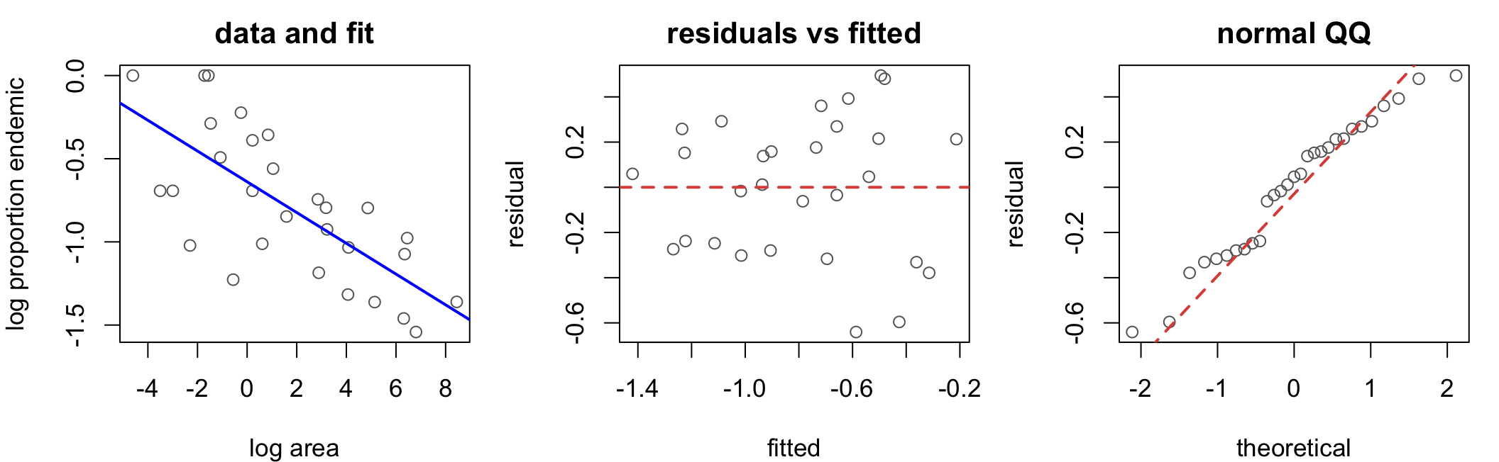
Looks good, but it’s a little less clear what we’re really checking, and that’s the cost of transformations — less interpretability.