Applied Linear Models

STAT3530 Fall 2026

The linear model

We can write the linear model as

\[Y = X\beta + \epsilon\,, \quad \mathbb{E}[\epsilon] = 0\,, \quad \text{Var}[\epsilon] = \sigma^2 I\]

where everything is a vector or matrix

  • \(Y\) is an \(n\times 1\) vector
  • \(X\) is an \(n\times 2\) matrix
  • \(\beta\) is a \(2\times 1\) vector
  • \(\epsilon\) is an \(n\times 1\) random vector
  • \(I\) is the \(n\times n\) identity matrix.

\[\underbrace{\left[\begin{array}{c} Y_1 \\ Y_2 \\ \vdots \\ Y_n \end{array}\right]}_{Y} = \underbrace{\left[\begin{array}{cc} 1 &x_1 \\ 1 &x_2 \\ \vdots \\ 1 &x_n \end{array}\right] \left[\begin{array}{c} \beta_0 \\ \beta_1 \end{array}\right]}_{X\beta} + \underbrace{\left[\begin{array}{c} \epsilon_1 \\ \epsilon_2 \\ \vdots \\ \epsilon_n \end{array}\right]}_\epsilon\]

The least squares criterion

Recall that the least squares estimates minimize \[SSE(\beta_0, \beta_1) = \sum_{i = 1}^n \left( Y_i - \beta_0 - \beta_1 x_i \right)^2\]

Express this as the inner product \[SSE(\beta) = (Y - X\beta)^T (Y - X\beta)\]

Two approaches to finding the minimizer:

  1. calculus
  2. geometry

A dash of vector calculus

The gradient is the vector equivalent of a derivative.

If \(x \in \mathbb{R}^p\) and \(f(x)\) is a real-valued function the gradient is \[\nabla f(x) = \left[\begin{array}{cccc} \frac{\partial f}{\partial x_1} &\frac{\partial f}{\partial x_2} &\cdots &\frac{\partial f}{\partial x_p} \end{array}\right]^T \quad\text{where}\quad \frac{\partial f}{\partial x_j} = \frac{d}{dx_j}f(x)\]

Example:

\[\begin{align*} f(x) &= x_1^2 + 3 x_2 \\ \nabla f(x) &= \left[\begin{array}{cc} 2x_1 &3 \end{array}\right]^T \end{align*}\]

Your turn: If \(f(x) = 4x_1 + 5x_2\) then \(\nabla f(x) = \left[\hspace{1in}\right]^T\)

The calculus approach

Let \(A \in \mathbb{R}^{p\times p}\) be a symmetric matrix and \(a, x \in \mathbb{R}^p\) be vectors. Two rules: \[\nabla a^T x = \nabla x^T a = a \quad\text{and}\quad \nabla x^T A x = 2Ax\]

Now expand SSE \[\begin{align*} SSE(\beta) &= (Y - X\beta)^T (Y - X\beta) \\ &= (Y^T - \beta^T X^T)(Y - X\beta) \\ &= Y^T Y - \underbrace{Y^T X}_{a^T}\beta - \beta^T \underbrace{X^T Y}_{a} + \beta^T \underbrace{X^T X}_{A} \beta \end{align*}\]

And apply the rules to get \[\nabla SSE(\beta) = -2 X^T Y + 2 X^T X \beta = 0 \quad\Longrightarrow\quad X^T X \beta = X^T Y\]

The least squares estimator

\[\nabla SSE(\beta) = 0 \quad\Longrightarrow\quad X^T X \beta = X^T Y\]

If \(X^T X\) is invertible then \(SSE\) has a minimum at \[\beta = (X^T X)^{-1} X^T Y\] We will verify that this is a minimum later.

The minimizer is the least squares estimator, which we denote: \[\hat\beta = (X^T X)^{-1} X^T Y\]

The geometry approach

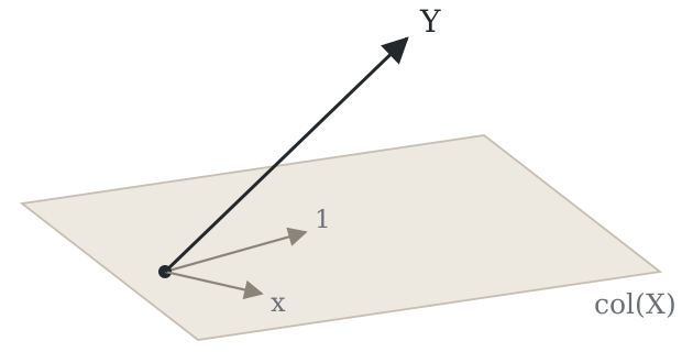
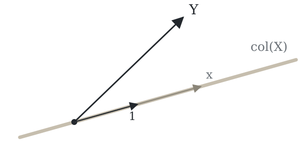
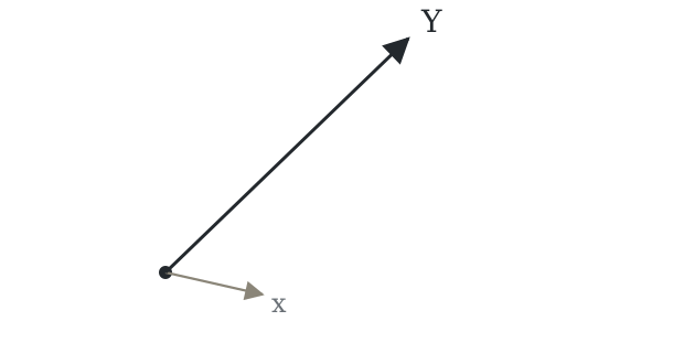
Data are \(x, Y \in \mathbb{R}^n\).

Picture them in n-dimensional space.

The geometry approach

Now add the vector of ones \(\mathbf{1}\).

\(\mathbf{1}\) and \(x\) span a two-dimensional space. That’s the column space of \(X\).

\[X = \left[\begin{array}{cc} 1 &x_1 \\ 1 &x_2 \\ \vdots \\ 1 &x_n \end{array}\right]\]

Is it always two-dimensional?

Why or why not?

The geometry approach

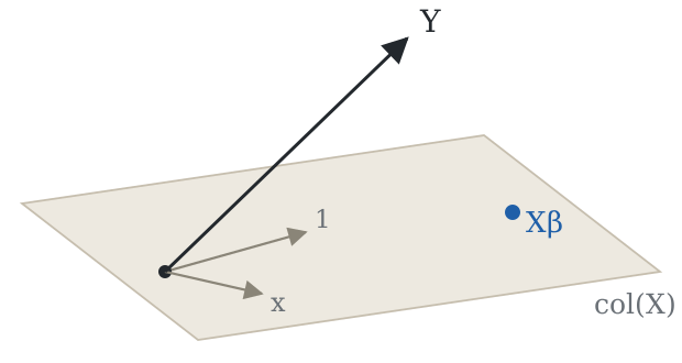
Think of \((\beta_0, \beta_1)\) as coordinates of a point \[X\beta \in \text{col}(X)\]

The geometry approach

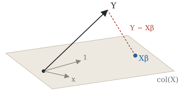
Think of \((\beta_0, \beta_1)\) as coordinates of a point \[X\beta \in \text{col}(X)\]

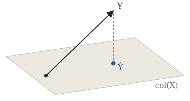
and picture the residual vector \(Y-X\beta\).

Observe that

\[SSE(\beta) = (Y - X\beta)^T (Y - X\beta)\]

is precisely its squared length.

So to minimize, find the point closest to \(Y\).

The geometry approach

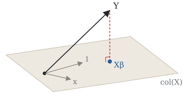
The residual vector will be orthogonal to \(\text{col}(X)\) at that point.

Algebraically, orthogonality means

\[X^T \left(Y - X\beta\right) = 0\]

So the minimizer satisfies:

\[X^T Y = X^T X \beta\]

Giving:

\[\hat\beta = (X^T X)^{-1} X^T Y\]

This must be a minimum by the Pythagorean theorem.

The geometry approach

So now if you want to sound fancy:

The least squares estimate is simply the orthogonal projection of the data onto the linear subspace spanned by the predictors.

Is \(X^T X\) invertible?

Two facts:

  1. A square matrix \(A \in \mathbb{R}^{p\times p}\) is invertible just in case \(\text{rank}(A) = p\)
  2. For any matrix \(X\), \(\text{rank}(X^T X) = \text{rank}(X)\)

Recall that

\[X = \left[\begin{array}{cc} 1 &x_1 \\ 1 &x_2 \\ \vdots &\vdots\\ 1 &x_n \end{array}\right]\]

So \(X^T X\) is invertible just in case \(\text{rank}(X) = \_\_\_\_\_\)

i.e., just in case \(X\) is f______ r______.

Is \(X\) full rank?

Need to check that the columns are linearly independent. We have:

\[X = \left[\begin{array}{cc} 1 &x_1 \\ 1 &x_2 \\ \vdots &\vdots\\ 1 &x_n \end{array}\right]\]

When would the columns NOT be linearly independent?

Full rank, geometrically

\(X\) is rank-degenerate exactly when \(x = c\mathbf{1}\).

Interestingly, you can still project and get \[X\beta = \bar{Y}\] but this does not uniquely determine \(\beta\).

So the model \(Y_i = \beta_0 + \beta_1 c + \epsilon_i\) collapses to \(Y_i = \mu + \epsilon_i\) and only \(\mu\) is identifiable.

Least squares summary

So with the linear model in matrix form

\[Y = X\beta + \epsilon\]

the least squares estimate minimizes

\[SSE(\beta) = (Y - X\beta)^T (Y - X\beta) = \|Y - X\beta\|^2\]

and we have shown that the minimizer is

\[\hat{\beta} = (X^T X)^{-1} X^T Y\]

provided \(X\) is full rank.

Note that this is pure optimization; there are no statistical assumptions.

Now, the statistical perspective

Let’s distinguish

  • estimand: the thing to estimate
  • estimator: a way to estimate it
  • estimate: value from a specific dataset

So for example

  • estimand: \(\beta_1\)
  • estimator: \(rs_y/s_x\)
  • estimate: -1.191

Estimands are fixed but unknown. Estimates are fixed and known.

But estimators are functions of data, and therefore random.

Properties of \(\hat{\beta}\)

The least squares estimator is a random vector

\[\hat\beta = \underbrace{(X^T X)^{-1}X^T}_{\text{fixed}} \underbrace{Y}_{\text{random}}\]

Under the model \(Y = X\beta + \epsilon\): \[\mathbb{E}[\epsilon] = 0 \quad\Longrightarrow\quad \mathbb{E}[Y] = \mathbb{E}[X\beta + \epsilon] = X\beta + \mathbb{E}[\epsilon] = X\beta \\\]

And therefore: \[\begin{align} \mathbb{E}\left[\hat\beta\right] = \mathbb{E}\left[(X^T X)^{-1}X^T Y\right] = (X^T X)^{-1}X^T \mathbb{E}[Y] = (X^T X)^{-1}X^T X\beta = \beta \end{align}\]

We say the estimator is unbiased: its average value across datasets is the estimand.

Properties of \(\hat{\beta}\): variance

Further \[\text{var}[\epsilon] = \sigma^2 I \quad\Longrightarrow\quad \text{var}[Y] = \text{var}[X\beta + \epsilon] = \text{var}[\epsilon] = \sigma^2 I\]

And therefore \[\begin{align} \text{var}\left[\hat\beta\right] &= \text{var}\left[(X^T X)^{-1}X^T Y\right] \\ &= \left[(X^T X)^{-1}X^T\right] \text{var}[Y] \left[(X^T X)^{-1}X^T\right]^T \\ &= \left[(X^T X)^{-1}X^T\right] (\sigma^2I) \left[(X^T X)^{-1}X^T\right]^T \\ &= \sigma^2 (X^T X)^{-1}X^T X (X^T X)^{-1} \\ &= \sigma^2 (X^T X)^{-1} \end{align}\]

The variance quantifies sampling variability.

Check your understanding: what are the dimensions of \(\sigma^2 (X^T X)^{-1}\)?

Simulating \(\hat\beta\)

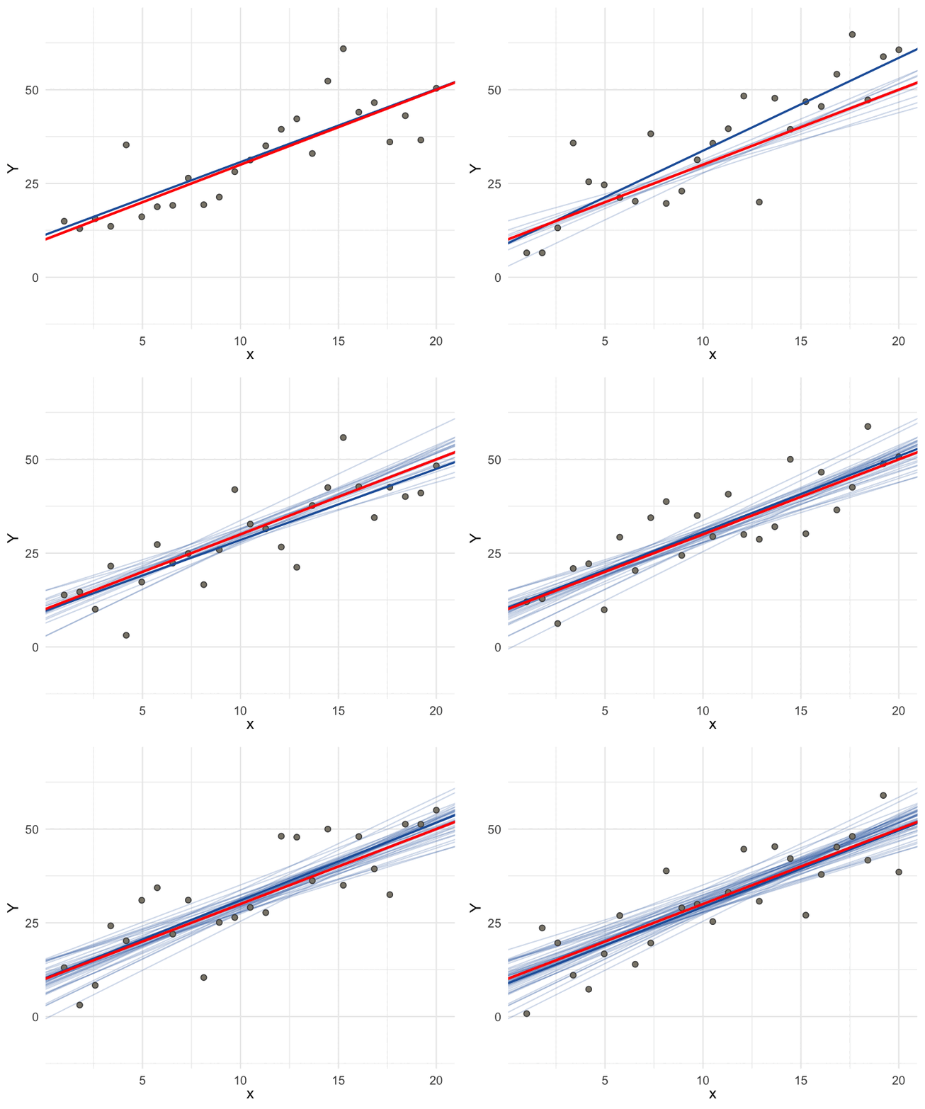
Fix \(x\), simulate 50 datasets from \(Y_i = 10 + 2 x_i + \epsilon_i\), and estimate \(\beta\) for each one.

The average of the fitted lines falls on the true line. That’s unbiasedness:

\[\mathbb{E}[\hat\beta] = \beta\]

The spread of the fitted lines is determined by the variance:

\[\text{var}[\hat\beta] = \sigma^2(X^TX)^{-1}\]

Simulating \(\hat\beta\)

Estimates from the first ten simulations:

      intercept    slope
 [1,] 11.246602 1.947468
 [2,] 12.512949 1.708344
 [3,] 14.958101 1.445810
 [4,]  8.682867 2.046064
 [5,]  9.669574 2.168417
 [6,]  9.303270 1.971275
 [7,]  7.181456 2.225554
 [8,]  9.213057 2.116058
 [9,]  2.836404 2.491463
[10,] 10.859322 1.703452

Now consider

# average simulated estimate
apply(B, 1, mean)
intercept     slope 
 9.979620  2.004444 
# variances of simulated estimates
apply(B, 1, var)
  intercept       slope 
11.66160516  0.08338812 
# theoretical variance
64*solve(t(X) %*% X)
                       x
  11.2202514 -0.82478585
x -0.8247859  0.07855103

Questions:

  1. Which numbers suggest estimates are unbiased?
  2. What error variance was used in the simulations?
  3. What is -0.8248? How would you approximate it?

Wait, the estimators are correlated?

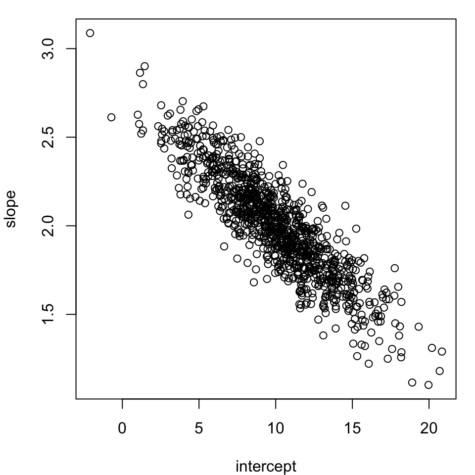
The plot shows simulated pairs \(\left(\hat\beta_0, \hat\beta_1\right)\).

Each point is one estimate.

cor(B['slope', ], B['intercept', ])
[1] -0.883547

Why would this happen?

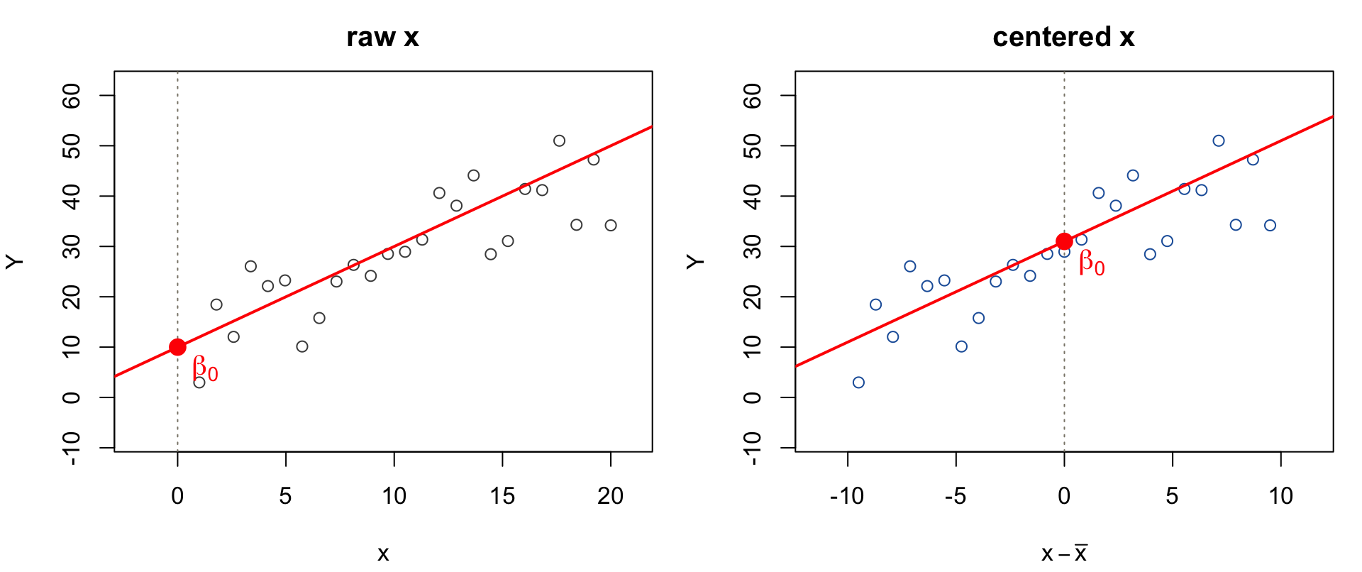
Centering the predictor

If we instead fit

\[Y_i = \beta_0 + \beta_1 (x_i - \bar{x}) + \epsilon_i\] then \(\beta_0\) represents the mean of \(Y\) at \(\bar{x}\) and the estimators become uncorrelated.

Centering the predictor

If we instead fit

\[Y_i = \beta_0 + \beta_1 (x_i - \bar{x}) + \epsilon_i\]

then mathematically

\[X = \left[\begin{array}{cc} 1 & x_1 - \bar{x} \\ 1 & x_2 - \bar{x} \\ \vdots &\vdots \\ 1 & x_n - \bar{x} \\ \end{array}\right] = \left[\begin{array}{cc}\mathbf{1} & (I - \frac1n\mathbf{11}^T)\,x\end{array}\right]\]

and it is straightforward to show (HW2) that \[X^T X = \left[\begin{array}{cc} n &0 \\ 0 &(n - 1)s^2_x \end{array}\right] \quad\text{and thus}\quad (X^T X)^{-1} = \left[\begin{array}{cc} \frac{1}{n} & 0 \\ 0 & \frac{1}{(n - 1)s^2_x} \end{array}\right]\]

Centering the predictor

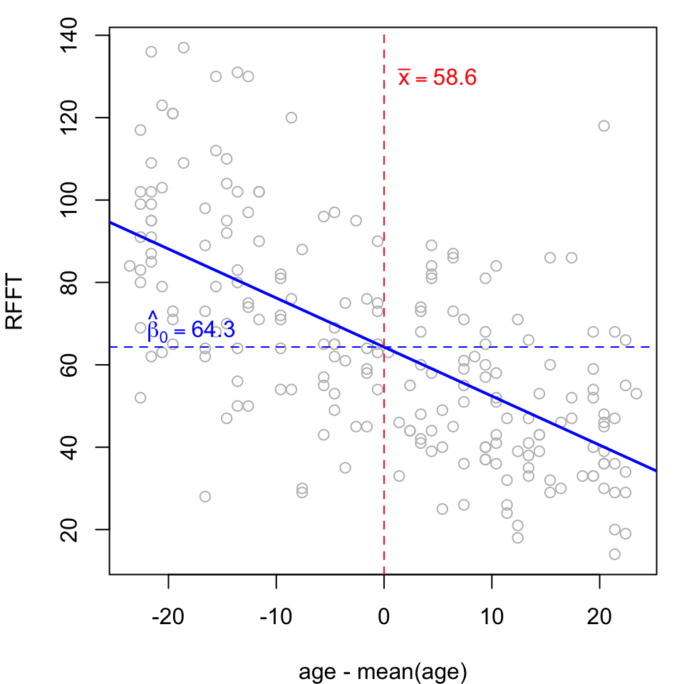
For example, centering age in the RFFT model:

# fit with centered predictor
fit <- lm(rfft ~ I(age - mean(age)), 
          data = prevend)
# inspect
fit

Call:
lm(formula = rfft ~ I(age - mean(age)), data = prevend)

Coefficients:
       (Intercept)  I(age - mean(age))  
            64.322              -1.191  

Your turn:

  1. Interpret the intercept \(\hat{\beta}_0\).
  2. What would happen if we also centered \(Y\)?

Optimality of least squares

So far we know that \(\mathbb{E}[ \hat{\beta} ] = \beta\) and \(\text{Var}[\hat{\beta}] = \sigma^2 (X^T X)^{-1}\). Could we do better?

We can’t improve on the bias, so “better” here would mean smaller variance.

Writing \(\hat{\beta} = AY\) with \(A = (X^TX)^{-1}X^T\), we see it is a linear function of \(Y\).

Gauss-Markov theorem. For any unbiased estimator of the form \(AY\), we have that \(\text{var}[AY] \succeq \text{var}[\hat{\beta}]\) under the model \(Y = X\beta + \epsilon\) with \(\mathbb{E}[\epsilon] = 0\) and \(\text{Var}(\epsilon) = \sigma^2 I\).

For a proof, see Rencher & Schaalje, Linear Models in Statistics.

So the least squares estimator is the best linear unbiased estimator, or BLUE for short.

Fitted values

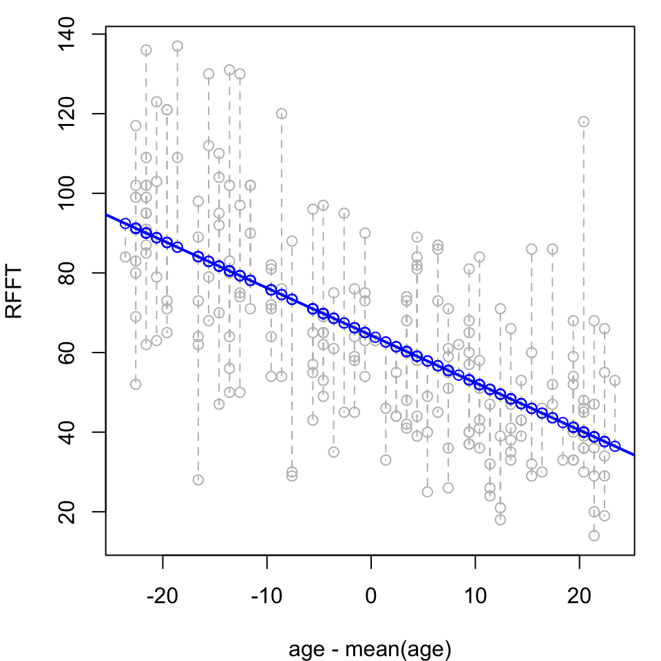
We call \(\hat{Y} = X\hat\beta\) the “fitted values”.

Observe that \[\hat{Y} = \underbrace{X (X^TX)^{-1}X^T}_{H}\; Y\] where \(H\) is an orthogonal projection.

The hat matrix

We call \(H\) the “hat matrix” because it puts a hat on \(Y\): \[\hat{Y} = HY\]

\(H\) is an orthogonal projection in the formal sense, meaning it is

  • symmetric: \(H^T = H\)
  • idempotent: \(HH = H\)

The residuals can be written compactly using the hat matrix: \[e = Y - HY = (I - H)Y\]

and \(I - H\) is also a projection (see handout), specifically onto the orthogonal complement of \(\text{col}(X)\) in \(\mathbb{R}^n\), which we denote by \(\text{col}(X)^\perp\).

Estimating \(\sigma^2\)

Variance is always a little trickier.

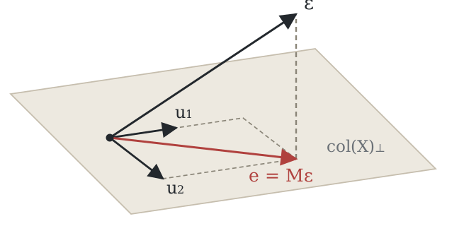
Now since \((I - H)X = 0\), the residual vector is a projection of \(\epsilon\) onto \(\text{col}(X)^\perp\):

\[e = (I - H)Y = (I - H)(X\beta + \epsilon) = (I - H) \epsilon\]

which we can re-express as \[(I - H)\,\epsilon = \sum_{j} (u_j^T\, \epsilon)\, u_j\] where \(u_1, \dots, u_{n-2}\) is an orthonormal basis.

Estimating \(\sigma^2\)

Now the residual variance is proportional to \(\|e\|^2\). As a matter of algebra \[\|e\|^2 = [(I - H)\,\epsilon]^T [(I - H)\, \epsilon] = \sum_{j} (u_j^T\,\epsilon)^2\]

Now since \(\mathbb{E}[u_j^T\epsilon] = 0\) we have that \(\text{var}[u_j^T\epsilon] = \mathbb{E}[(u_j^T \epsilon)^2]\), and then \[\mathbb{E}\left[\|e\|^2\right] = \sum_j \text{var}\left(u_j^T\,\epsilon\right) = \sum_j u_j^T\, (\sigma^2 I)\, u_j = \sum_j \sigma^2 u_j^T u_j = (n - 2)\, \sigma^2\]

And finally, we obtain an unbiased estimate of the residual variance \[\hat{\sigma}^2 = \frac{1}{n - 2}\, \|e\|^2\]

Uncertainty quantification

All told, we now have

  • least squares estimates \(\hat{\beta} = (X^T X)^{-1} X^T Y\)
  • theoretical variance \(\text{var}\left[\hat\beta\right] = \sigma^2 (X^TX)^{-1}\)
  • unbiased error variance estimator \(\hat{\sigma}^2 = (n - 2)^{-1} \|e\|^2\)

Put these together and we get point estimates \(\hat{\beta}\) with standard errors given by \[\widehat{\text{var}}\left(\hat{\beta}\right) = \hat{\sigma}^2 (X^T X)^{-1}\]

i.e., \[SE\left(\hat{\beta}_j\right) = \sqrt{\hat{\sigma}^2 \left( (X^T X)^{-1} \right)_{jj}}\]

Interpreting variance estimates

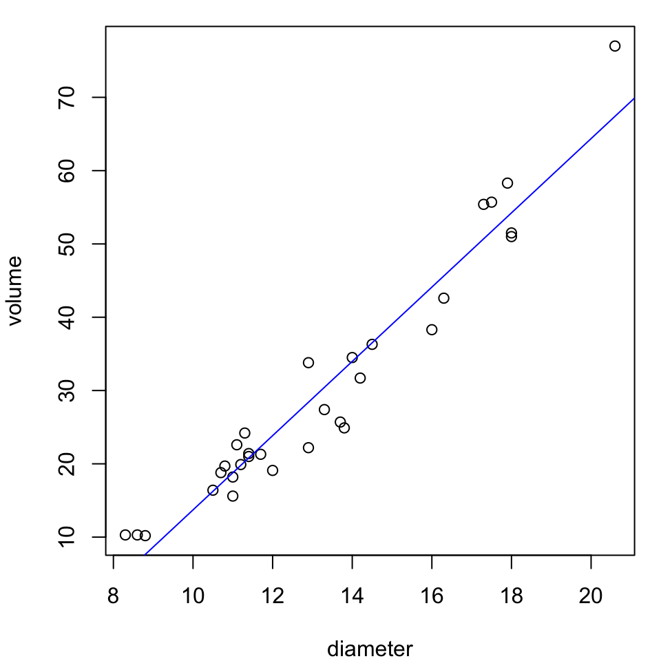
Timber volume (cubic ft) vs. diameter (in) for 31 felled cherry trees.

# fit the model
fit <- lm(volume ~ diameter, data = cherry)

# coefficient estimates
coef(fit)
(Intercept)    diameter 
 -36.943459    5.065856 
# variance parameter estimate
sigma(fit)
[1] 4.251988
# estimated variance-covariance matrix
vcov(fit)
            (Intercept)    diameter
(Intercept)  11.3242005 -0.81073976
diameter     -0.8107398  0.06119536
  • across samples, the intercept estimate varies by an estimated 3.365 on average
  • across samples, the slope estimate varies by an estimated 0.247 on average

Your turn

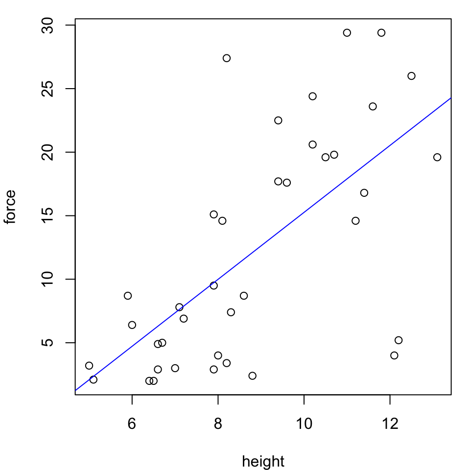
Claw height and closing force of 38 predatory crabs.

# fit the model
fit <- lm(force ~ height, data = crab)

# coefficient estimates
coef(fit)
(Intercept)      height 
 -11.086902    2.634823 
# variance parameter estimate
sigma(fit)
[1] 6.89171
# estimated variance-covariance matrix
vcov(fit)
            (Intercept)     height
(Intercept)   21.366599 -2.2825772
height        -2.282577  0.2589965

Interpret each of the estimates above:

  • coefficients \(\hat{\beta}\)
  • error variance \(\hat{\sigma}^2\)
  • coefficient variances \(\hat{\sigma}^2 (X^T X)^{-1}\)

One last assumption

So far we have that under the model \[Y = X\beta + \epsilon\,, \quad \mathbb{E}[\epsilon] = 0\,, \quad \text{Var}[\epsilon] = \sigma^2 I\] the least squares estimates are BLUE with \(\text{var}(\hat\beta) = \sigma^2 (X^T X)^{-1}\).

If in addition we assume the errors are normal, we get that \[\epsilon \sim N(0, \sigma^2 I) \quad\Longrightarrow\quad \hat\beta \sim N(\beta\,, \sigma^2 (X^T X)^{-1})\]

This provides a basis for statistical inference on \(\beta\)
  • confidence intervals
  • hypothesis testing