Applied Linear Models

STAT3530 Fall 2026

Welcome!

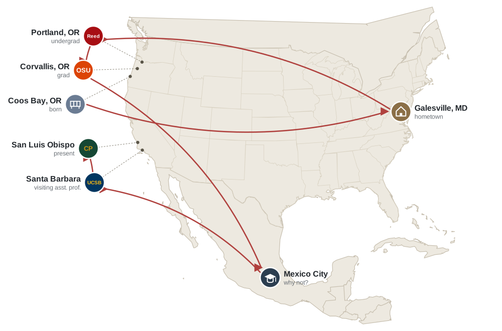
I’m Trevor. This is how I got here.

Note to self: go over syllabus.

We have a small group so let’s do icebreakers:

  • name
  • hometown
  • hobby or interest
  • book recommendation
  • goal for the term/year?

Regression review

Correlation

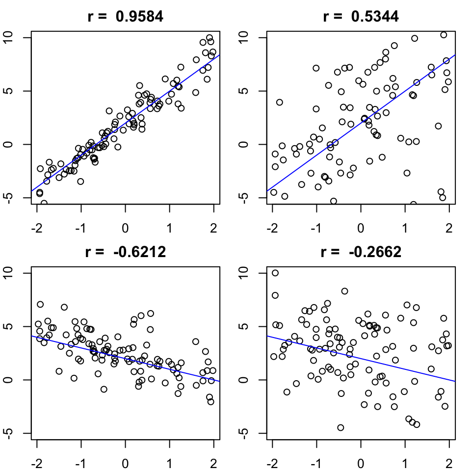
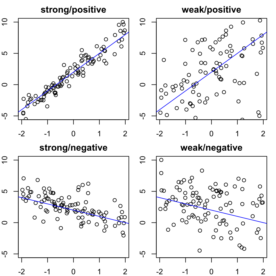
Measures direction and strength of linear relationship.

\[r = \frac{\sum_i (x_i - \bar{x})(y_i - \bar{y})}{(n-1) \times s_x \times s_y}\]

  • sign indicates direction of relationship
  • magnitude indicates strength
  • between -1 and 1

The classic caveat

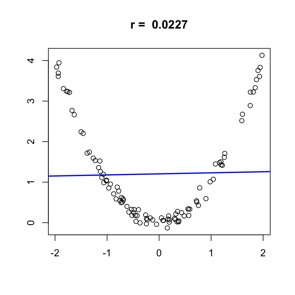
Correlation only measures the strength of linear relationships.

  • \(r\approx0 \not\Leftrightarrow\) no relationship
  • visualize whenever possible

More on nonlinear relationships later.

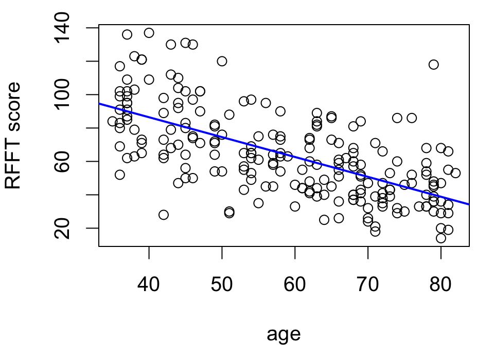
Ruff Figural Fluency Test (RFFT)

Measures nonverbal fluency and executive cognitive function on 0-175 scale.

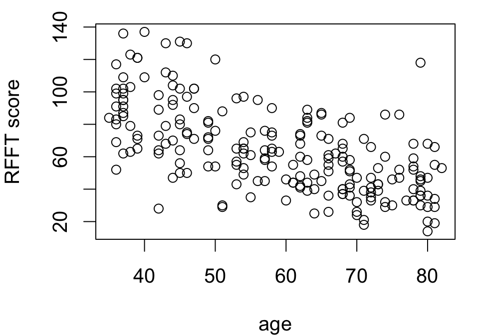
Data from \(n = 208\) observations show:

  • moderate, negative linear trend with age
  • \(r = -0.6359\)

\[\text{Model:}\qquad\text{RFFT}_i = \beta_0 + \beta_1 \text{age}_i + \epsilon_i \quad\text{for}\quad i = 1, \dots, 208\]

To “fit” this model, we need to find values for the regression coefficients \(\beta_0, \beta_1\).

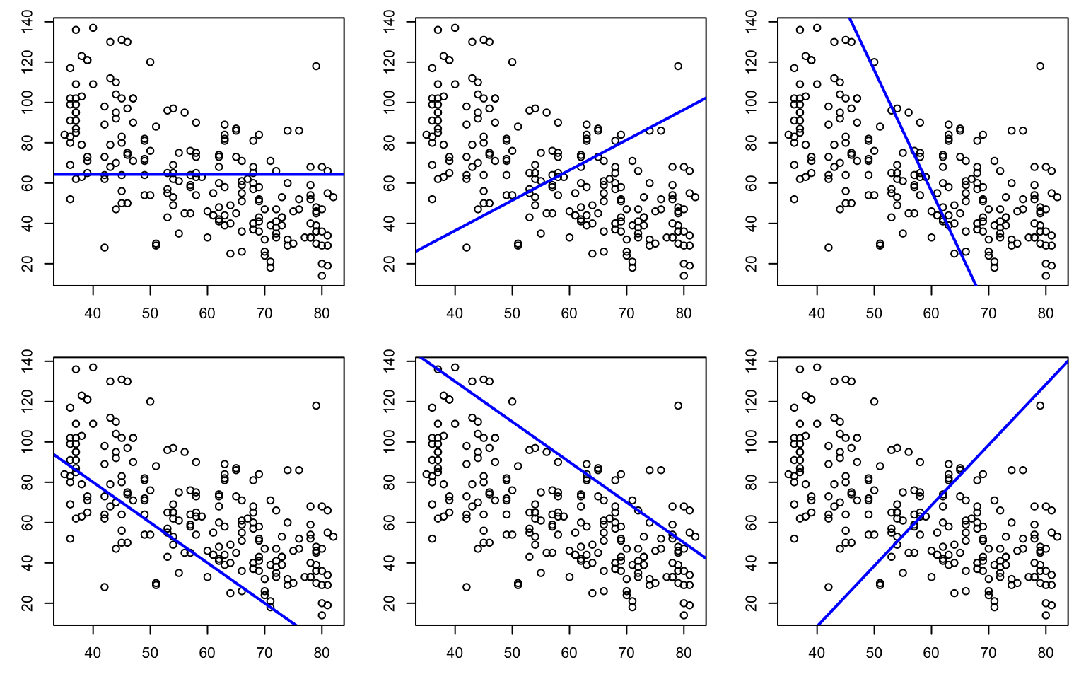
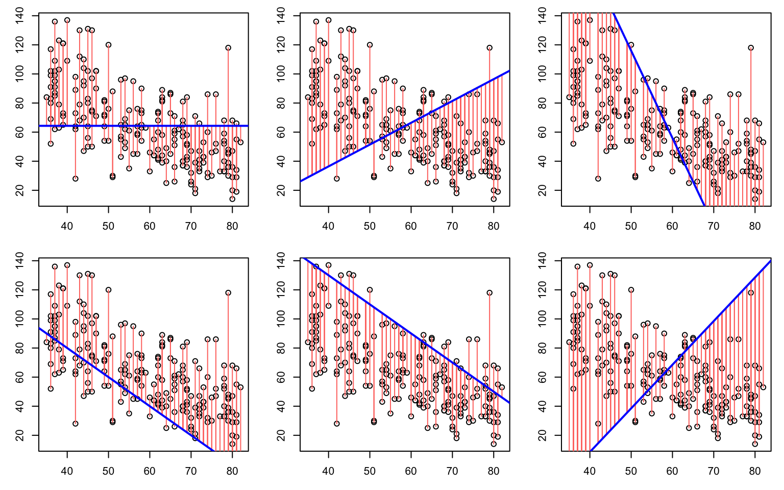
Some possible fits

None of these are good. Why not?

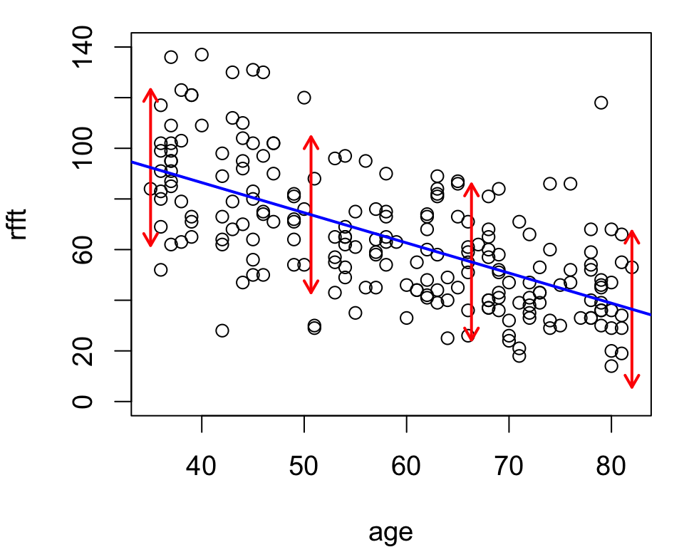
Model residuals

The residuals are too big. Smaller is better.

Least squares estimation

Rewrite the model in the form \[Y_i = \beta_0 + \beta_1 x_i + \epsilon_i\,, \qquad i = 1, \dots, 208\]

Given estimates \(\hat\beta_0, \hat\beta_1\), the residuals are \(\color{red}{e_i} = Y_i - \hat\beta_0 - \hat\beta_1 x_i\). So we minimize: \[SSE(\beta_0, \beta_1) = \sum_{i = 1}^n \left( Y_i - \beta_0 - \beta_1 x_i \right)^2\] Analytic solution:

\[\begin{align*} 0 &= \frac{d}{d\beta_0} \sum_{i = 1}^n \left( Y_i - \beta_0 - \beta_1 x_i \right)^2 = \cdots [\text{HW1}] \cdots \Rightarrow \hat\beta_0 = \bar{Y} - \beta_1 \bar{x} \\ 0 &= \frac{d}{d\beta_1} \sum_{i = 1}^n \left( [Y_i - \bar{Y}] - \beta_1 [x_i - \bar{x}] \right)^2 = \cdots [\text{HW1}] \cdots \Rightarrow \hat\beta_1 = r\frac{s_y}{s_x} \end{align*}\]

lm() in R

fit <- lm(rfft ~ age, data = prevend)
print(fit)

Call:
lm(formula = rfft ~ age, data = prevend)

Coefficients:
(Intercept)          age  
    134.098       -1.191  

This says the least squares estimates are

  • \(\hat\beta_0 = 134.098\)
  • \(\hat\beta_1 = -1.191\)

The error term

Since the model errors \(\epsilon_1, \dots, \epsilon_n\) are random, we don’t estimate them.

Instead we characterize them through the assumptions:

  1. mean zero
  2. standard deviation \(\sigma\)
  3. mutually independent

And then estimate the variance by \[\hat\sigma = \sqrt{\frac{1}{n-2} \sum_{i = 1}^n e_i^2}\]

sigma(fit)
[1] 20.51788

Model interpretation

The line represents an average; it is obviously false as a description of the observations.

Parameter interpretations:

  • \(\beta_0\): mean \(Y\) when \(x = 0\)
  • \(\beta_1\): change in mean \(Y\) per increment in \(x\)
  • \(\sigma^2\): unexplained variability in \(Y\) after accounting for \(x\)

For the RFFT model:

  • at age 0, mean RFFT is estimated to be 134.098
  • with each additional year of age, mean RFFT decreases by an estimated 1.191 points
  • after accounting for age, RFFT scores vary by 20.52 points on average

Your turn

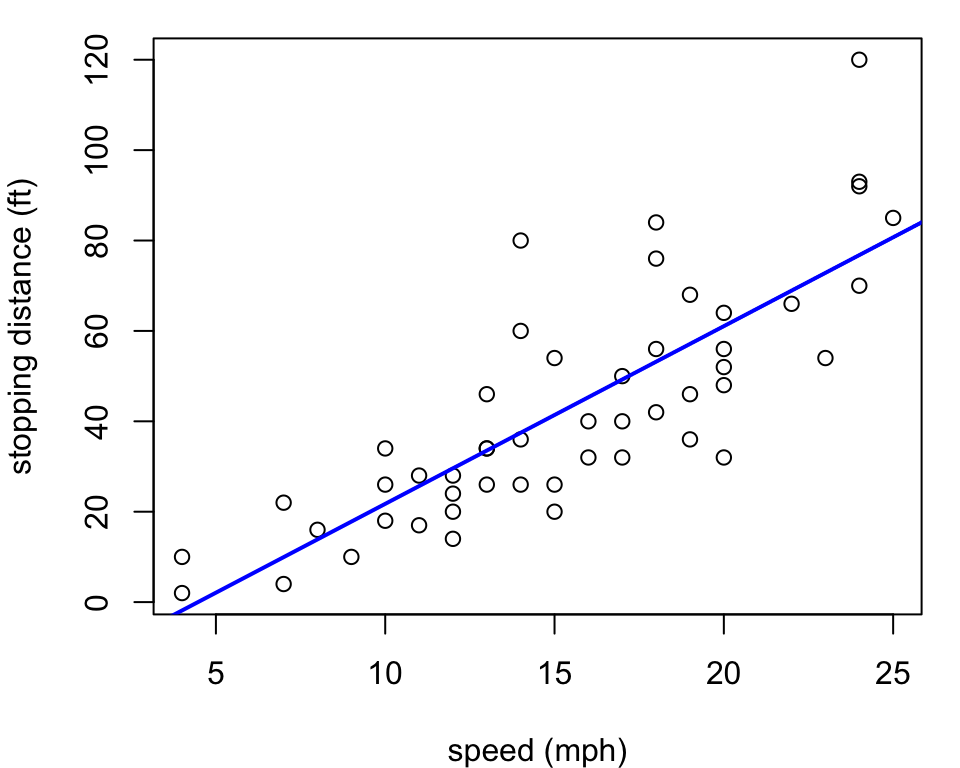
fit_cars <- lm(dist ~ speed, data = cars)
fit_cars

Call:
lm(formula = dist ~ speed, data = cars)

Coefficients:
(Intercept)        speed  
    -17.579        3.932  
sigma(fit_cars)
[1] 15.37959

First identify:

  • \(\hat\beta_0 = \hspace{1em}\)
  • \(\hat\beta_1 = \hspace{1em}\)
  • \(\hat\sigma = \hspace{1em}\)

Then interpret the estimates.

Starting points

So now we have:

  1. the (simple) linear model \(Y_i = \beta_0 + \beta_1 x_i + \epsilon_i\)
  2. how to estimate model parameters
  3. how to interpret estimates

In 3530 we will cover a variety of topics in connection with the general linear model

\[Y = X\beta + \epsilon\]

where each term is a vector or matrix.

Linear algebra review

Why linear algebra?

Provides a certain elegance.

  • Bookeeping: no complicated indexing, long summations, etc.
  • Generality: \(Y = X\beta + \epsilon\) describes a very wide class of models
  • Tractability: simplifies mathematical analysis

On that last point, note that with a little algebra we get:

\[\hat\beta_1 = \sum_{i=1}^n \underbrace{\frac{x_i - \bar{x}}{(n-1)s^2_x}}_{w_i} \, Y_i = \sum_{i=1}^n w_i Y_i = w^T Y \]

More detail later, but the least squares estimates are linear functions of the response \(Y\).

Vectors

An \(n\)-dimensional vector is a column of numbers

\[a = \left[\begin{array}{c} a_1 \\ \vdots \\ a_n \end{array}\right]\]

If its entries are real numbers we write \(a \in \mathbb{R}^n\).

For example, consider:

\[a = \left[\begin{array}{c} -1 \\ 0 \\ 2 \end{array}\right]\]

Your turn: \(a \in \hspace{1em}\)

Inner product

If \(a, b \in \mathbb{R}^n\) their inner product is the sum of the product of their entries:

\[\langle a, b \rangle = \sum_{i = 1}^n a_i \, b_i\]

For example, given

\[a = \left[\begin{array}{c} -1 \\ 0 \\ 2\end{array}\right],\quad b = \left[\begin{array}{c} 3 \\ 5 \\ 6\end{array}\right]\] The inner product is \[\langle a, b \rangle = (-1\cdot3) + (0\cdot5) + (2\cdot6) = 9 \]

Matrices

An \(n \times m\) matrix is an array of numbers

\[A = \left[\begin{array}{cccc} a_{11} &a_{12} &\cdots &a_{1m} \\ a_{21} &a_{22} &\cdots &a_{2m} \\ \vdots &\vdots &\ddots &\vdots \\ a_{n1} &a_{n2} &\cdots &a_{nm} \end{array}\right]\]

We sometimes write \(A_{n\times m}\) to indicate the dimensions explicitly and \(A = \{a_{ij}\}\) to indicate the indexing explicitly. If its entries are real numbers we write \(A \in \mathbb{R}^{n\times m}\).

For example:

\[A = \left[\begin{array}{ccc} 1 &0 &3\\ 4 &-2 &0 \end{array}\right]\]

Your turn: \(A \in \hspace{1em}\) and \(A_{\hspace{1em}\times\hspace{1em}}\)

Matrix transpose

If \(A = \{a_{ij}\}\) is a matrix, its transpose is \(A^T = \{a_{ji}\}\). For example:

\[A = \left[\begin{array}{ccc} 1 &0 &3\\ 4 &-2 &0 \end{array}\right],\qquad A^T = \left[\begin{array}{cc} 1 &4 \\ 0 &-2 \\ 3 &0 \end{array}\right]\]

Observe that vectors are matrices with column dimension 1. If

\[a = \left[\begin{array}{c} a_1 \\ \vdots \\ a_n \end{array}\right]\] then \(a\) is an \(n \times 1\) matrix. Its transpose is the \(1 \times n\) matrix

\[a^T = \left[\begin{array}{ccc} a_1 &\cdots &a_n \end{array}\right]\] which we call an \(n-\)dimensional row vector.

Row and column representations

We can write a matrix in terms of its columns or in terms of its rows. For example, if

\[A = \left[\begin{array}{ccc} 1 &0 &3\\ 4 &-2 &0 \end{array}\right]\]

then we can write either the column representation

\[A = \left[\begin{array}{ccc} a_1 &a_2 &a_3 \end{array}\right] \quad\text{where}\quad a_1 = \left[\begin{array}{c} 1 \\ 4 \end{array}\right],\, a_2 = \left[\begin{array}{c} 0 \\ -2 \end{array}\right],\, a_3 = \left[\begin{array}{c} 3 \\ 0 \end{array}\right]\]

or the row representation

\[A = \left[\begin{array}{c} a_1^T \\ a_2^T \end{array}\right] \quad\text{where}\quad a_1^T = \left[\begin{array}{ccc} 1 &0 &3 \end{array}\right] \quad\text{and}\quad a_2^T = \left[\begin{array}{ccc} 4 &-2 &0 \end{array}\right]\]

Matrix product

If \(A_{n\times m}, B_{m\times p}\) are matrices, their product is the \(n \times p\) matrix with \((i,j)\)th entry \[AB = \left\{ \sum_{k=1}^m a_{ik} b_{kj} \right\} = \left\{ a_i^Tb_j\right\}\]

Note that \(a_i^T b_j\) is the inner product of the \(i\)th row of \(A\) with the \(j\)th column of \(B\).

For example, \[\underbrace{\left[\begin{array}{ccc} \color{blue}{1} &\color{blue}{0} &\color{blue}{3}\\ 4 &-2 &0 \end{array}\right]}_A\, \underbrace{\left[\begin{array}{cc} \color{blue}{0} &1 \\ \color{blue}{-1} &2 \\ \color{blue}{1} &0 \end{array}\right]}_{B} = \underbrace{\left[\begin{array}{cc} \color{blue}{3} &1 \\ 2 &0 \end{array}\right]}_{AB}\] Your turn: what is the \((1,1)\) entry of \(BA\)?

Matrix products and dimensions

\(AB\) exists just in case column dimension of \(A\) = row dimension of \(B\).

So if \(A_{3\times 2}, B_{3\times 4}\) are matrices then:

  • \(A^TB\) is \(2\times 4\)
  • \(B^TA\) is \(4\times 2\)
  • none of \(AB, BA, AB^T, BA^T, A^T B^T, B^T A^T\) are defined

In fact, one can check that \(A^T B\) and \(B^T A\) are transposes. In general, one has that \[(AB)^T = \left(B^TA^T\right)\] whenever the product exists.

Square matrices

An \(n \times n\) matrix (same row and column dimensions) is called “square”.

A square matrix \(A\) is:

  • symmetric if \(A^T = A\)
  • idempotent if \(AA = A\)

An identity matrix is a square matrix with ones along the diagonal: \[I_n = \left[\begin{array}{cccc} 1 &0 &\cdots &0 \\ 0 &1 &\cdots &0 \\ \vdots &\vdots &\ddots &\vdots \\ 0 &0 &\cdots &1 \end{array}\right]\] We usually write \(I\) plainly as dimensions are typically clear from context. It is called the identity matrix because, for any \(A_{n\times m}\), we have \(I_n A = A\) and \(AI_m = A\).

Matrix inversion

For a square matrix \(A_{n\times n}\), the inverse \(A^{-1}\) is the matrix satisfying \[AA^{-1} = A^{-1}A = I\] if it exists. If so, we say \(A\) is “invertible”.

Note the definition implies that \((A^T)^{-1} = (A^{-1})^T\).

Linear independence

Vectors \(a_1, \dots, a_m \in \mathbb{R}^n\) are linearly independent if \[c_1 a_1 + c_2 a_2 + \cdots + c_m a_m = 0 \quad\Longrightarrow\quad c_1 = c_2 = \cdots = c_m = 0\]

For example, if \[A = \left[\begin{array}{ccc} 1 &0 &3\\ 4 &-2 &0 \end{array}\right]\] the columns are not independent since \[-3\left[\begin{array}{c} 1 \\ 4\end{array}\right] -6\left[\begin{array}{c} 0 \\ -2\end{array}\right] +\left[\begin{array}{c} 3 \\ 0\end{array}\right] = \left[\begin{array}{c} 0 \\ 0\end{array}\right] \qquad\text{that is,}\qquad a_3 = 3a_1 + 6a_2\]

Your turn: are \(a_1, a_3\) independent?

Matrix rank

If \(A \in \mathbb{R}^{n\times m}\), its column space is the linear subspace spanned by its columns \[\text{span}(a_1, \dots, a_m) = \left\{ c_1 a_1 + \cdots + c_m a_m \;:\; c_1, \dots, c_m \in \mathbb{R} \right\}\]

with dimension equal to the number of linearly independent columns.

The rank of \(A\) is the dimension of its column space \[\text{rank}(A) = \dim \left( \text{span}(a_1, \dots, a_m) \right)\] We always have \(\text{rank}(A) \leq \min(n, m)\); when equality holds we say \(A\) is “full rank”.

Consider again \[A = \left[\begin{array}{ccc} 1 &0 &3\\ 4 &-2 &0 \end{array}\right]\] Your turn: What is the rank of \(A\)? Is it full rank?

Random variables and vectors

Random variable

Variable: a term that takes different values.

Random variable: one whose values depend on chance.

An RV’s distribution describes the observation frequency of each value.

  • different samples \(\rightarrow\) different values
  • useful model for measurement error

A very simple statistical model

Measurements from a random sample = repeated independent observations of an RV

Distribution becomes a model for the data.

Formally, we write

\[Y_1, \dots, Y_{208} \stackrel{iid}{\sim} F\]

where

\[Y_i = i\text{th RFFT measurement}\]

to mean the measurements are independent and identically distributed (i.i.d.) RVs with common distribution \(F\).

Mean and variance

Distributions have a center and spread, just like data from a sample.

For an RV \(Y \sim F\), define

  • \(\mathbb{E}[Y]\): expected value or mean
  • \(\text{Var}[Y] = \mathbb{E}[(Y - \mathbb{E}[Y])^2]\): variance

Functions of random variables are themselves random variables. Fun facts:

  • expectation is linear: \(\mathbb{E}[aY + b] = a\mathbb{E}[Y] + b\)
  • variance is not (but close): \(\text{Var}[aY + b] = a^2 \text{Var}[Y]\)

Your turn: if \(\mathbb{E}[Y] = 2\), what is \(\mathbb{E}[3Y + 5]\)? What about \(\text{Var}[3Y + 5]\)?

The normal distribution

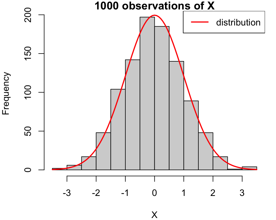
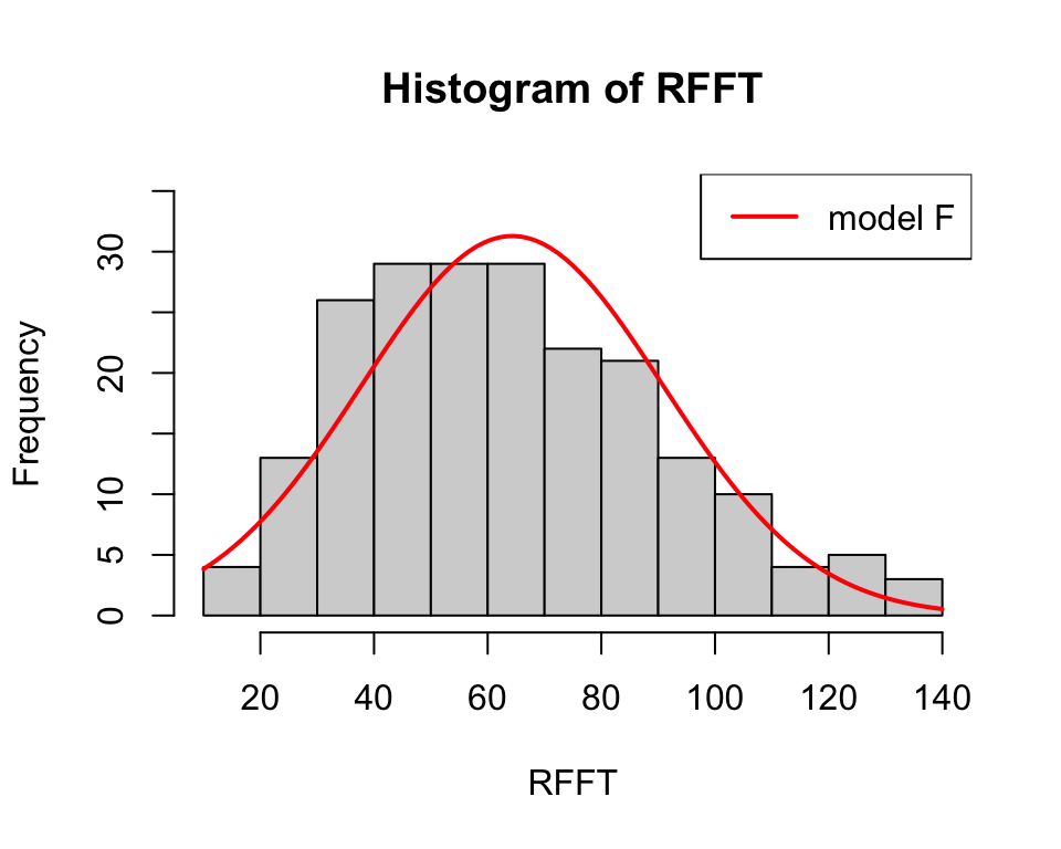
Those red curves are normal distributions.

We write

\[Y \sim N(\mu, \sigma^2)\]

to mean \(Y\) is normally distributed with

  • \(\mathbb{E}[Y] = \mu\)
  • \(\text{Var}[Y] = \sigma^2\)

Useful fact: \[aY + b \sim N(a\mu + b, a^2\sigma^2)\]

Your turn: if \(Y \sim N(\mu, \sigma^2)\), then \(Y - \mu \sim N(\hspace{1em}, \hspace{1em})\)

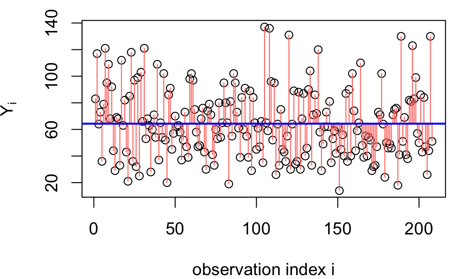
The very simple model, rewritten

The model you saw earlier for RFFT was \[Y_i \stackrel{iid}{\sim} N(\mu, \sigma^2)\]

or equivalently,

\[Y_i = \color{blue}{\mu} + \color{red}{\epsilon_i} \quad\text{where}\quad \epsilon_i \stackrel{iid}{\sim} N(0, \sigma^2)\] In other words: \[\text{RFFT} = \text{average} + \text{deviation}\]

Covariance

For dependent observations, covariance measures how two RVs vary together.

If \(Y_1, Y_2\) are RVs, we define

\[\text{Cov}[Y_1, Y_2] = \mathbb{E}\left[(Y_1 - \mathbb{E}[Y_1])(Y_2 - \mathbb{E}[Y_2])\right]\]

Facts:

  • \(\text{Cov}[Y, Y] = \text{Var}[Y]\)
  • \(\text{Cov}[Y_1, Y_2] = \text{Cov}[Y_2, Y_1]\)
  • \(\text{Cov}[aY_1 + b, Y_2] = a\text{Cov}[Y_1, Y_2]\)
  • if \(Y_1, Y_2\) are independent then \(\text{Cov}[Y_1, Y_2] = 0\)

Linearity properties

For any two random variables \(\color{blue}{Y_1}, \color{red}{Y_2}\) and any constants \(a, b, c\) we have

\[\mathbb{E}\left[a\color{blue}{Y_1} + b\color{red}{Y_2} + c\right] = a\,\mathbb{E}[\color{blue}{Y_1}] + b\,\mathbb{E}[\color{red}{Y_2}] + c\]

and

\[\text{Var}\left[a\color{blue}{Y_1} + b\color{red}{Y_2} + c\right] = a^2\text{Var}[\color{blue}{Y_1}] + b^2\text{Var}[\color{red}{Y_2}] + 2ab\,\text{Cov}[\color{blue}{Y_1}, \color{red}{Y_2}]\]

Note that if \(Y_1, Y_2\) are independent, \(\text{Cov}[Y_1, Y_2] = 0\) and we obtain

\[\text{Var}\left[aY_1 + bY_2 + c\right] = a^2\text{Var}[Y_1] + b^2\text{Var}[Y_2]\]

Random vectors

A random vector is a vector whose entries are random variables:

\[Y = \left[\begin{array}{ccc} Y_1 &\cdots &Y_n\end{array}\right]^T\]

Its mean vector and covariance matrix are defined by \[\mathbb{E}[Y] = \left[\begin{array}{c} \mathbb{E}[Y_1] \\ \vdots \\ \mathbb{E}[Y_n]\end{array}\right] \qquad\text{and}\qquad \text{Var}[Y] = \left\{\text{Cov}[Y_i, Y_j]\right\}\]

Linearity properties entail that for any fixed matrix \(A\) with conformal dimensions, \[\mathbb{E}[AY] = A\,\mathbb{E}[Y] \qquad\text{and}\qquad \text{Var}[AY] = A\,\text{Var}[Y]\,A^T\]

The very simple model, one last time

We can capture the features of the RFFT model in a single line

\[Y = \mu + \epsilon\,, \quad \mathbb{E}[\epsilon] = 0\,, \quad \text{Var}[\epsilon] = \sigma^2 I\] where everything is a vector or matrix:

  • \(\epsilon\) is an \(n\times 1\) random vector
  • \(\mu\) is an \(n\times 1\) fixed vector
  • \(I\) is the \(n\times n\) identity matrix.

If we adopt a normal model for the errors, we get the whole thing in a nutshell1 \[Y \sim N(\mu, \sigma^2 I)\]

The linear model in matrix form

Now consider the linear regression model \(\text{RFFT}_i = \beta_0 + \beta_1 \text{age}_{i} + \epsilon_i\).
In vector form: \[\left[\begin{array}{c} Y_1 \\ Y_2 \\ \vdots \\ Y_n \end{array}\right] = \beta_0 \left[\begin{array}{c} 1 \\ 1 \\ \vdots \\ 1 \end{array}\right] + \beta_1 \left[\begin{array}{c} x_1 \\ x_2 \\ \vdots \\ x_n \end{array}\right] + \left[\begin{array}{c} \epsilon_1 \\ \epsilon_2 \\ \vdots \\ \epsilon_n \end{array}\right]\]

Notice the linear portion can be written as a matrix product: \[\underbrace{\left[\begin{array}{c} Y_1 \\ Y_2 \\ \vdots \\ Y_n \end{array}\right]}_{Y} = \underbrace{\left[\begin{array}{cc} 1 &x_1 \\ 1 &x_2 \\ \vdots \\ 1 &x_n \end{array}\right] \left[\begin{array}{c} \beta_0 \\ \beta_1 \end{array}\right]}_{X\beta} + \underbrace{\left[\begin{array}{c} \epsilon_1 \\ \epsilon_2 \\ \vdots \\ \epsilon_n \end{array}\right]}_\epsilon\]

The linear model

Thus, we can write the linear model as:

\[Y = X\beta + \epsilon\,, \quad \mathbb{E}[\epsilon] = 0\,, \quad \text{Var}[\epsilon] = \sigma^2 I\]

where everything is a vector or matrix:

  • \(Y\) is an \(n\times 1\) vector
  • \(X\) is an \(n\times 2\) matrix
  • \(\beta\) is n \(2\times 1\) vector
  • \(\epsilon\) is an \(n\times 1\) random vector
  • \(I\) is the \(n\times n\) identity matrix.

What’s next: estimation

  • computing \(\hat\beta = \dots\) in terms of \(X, Y\)
  • properties of the least squares estimates